Strategies for Deploying Virtual Representations of the Built Environment
9 May 2020 Jon William Hand B.Sc., M.Arch., PhD, FIBPSA Energy Systems Research Unit, Department of Mechanical and Aerospace Engineering, University of Strathclyde, Glasgow, UK.
COPYRIGHT DECLARATION
The copyright of this publication belongs to the author under the terms of the United Kingdom Copyright Acts as qualified by the University of Strathclyde Regulation 3.49. Due acknowledgement must always be made of the use of any material contained in, or derived from, this publication.
Prior Editions
February
2006
September
2008
November
2010
June
2011
December
2013
November
2014
June
2015
March
2017
April
2018
It has been translated into Italian, French, Korean and portions into Greek (under separate copywrite).
A translation into Spanish is underway. A condensed version can be found here.
ACKNOWLEDGMENTS
This book could have been completed only within the exceptional group environment of the Energy Systems Research Unit of the University of Strathclyde in Glasgow Scotland. Where else could an architect work in and around a million lines of source code and then use the resulting virtual edifice to explore and support the design process and then turn the process on its head to return to the written page to explore strategies for its use.
CONVENTIONS USED
Where Appendices, other Sections or Exercises should be consulted before you proceed, the following icons are used:
If you are asked to study a particular section prior to continuing the subsequent text will assume that you have read the reference material.
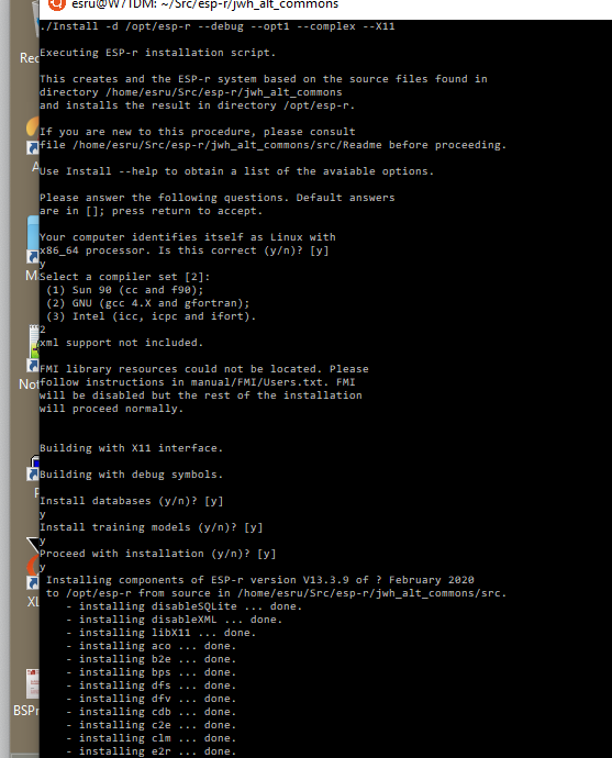
If you are asked to issue commands, for example to compile from source this is rendered as:
./Install ‐d /opt/esp-r ‐‐debug ‐‐complex --opt2
When describing a path through a menu structure the following convention is used: [Model Management] ‐> [browse/edit/simulate] ‐> [composition] ‐> [geometry & attribution] where the menu titled [Model Management] has an entry [browse/edit/simulate] which has an entry [composition].
There are grey corners in simulation tools and working practices that can so easily grow out of control and lead to calamity. These are highlighted via:
CFD is powerful. And also wrapped up in jargon which sounds like English. It is a place where dragons live. ESP‐r’s interface to CFD has a steep learning curve.
And there are many places where small differences in approach (and attitude) can have a significant impact. These are highlighted via:
QA works better if something that looks like a door, is named door and is composed of a type of construction which is associated with doors. Where attributes reinforce each other it is easy to notice if we get something wrong!
A word about ESP‐r interfaces
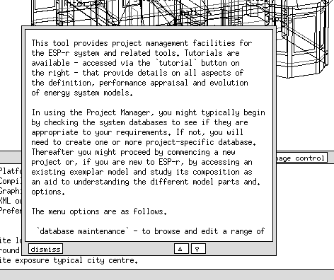
Strategies uses ESP-r for purposes of discussion. ESP‐r is under active development. On any given day there may several commits of code, documentation or model updates to the ESP‐r repository. Thus, references to facilities and interface elements may diverge somewhat from what is shown.
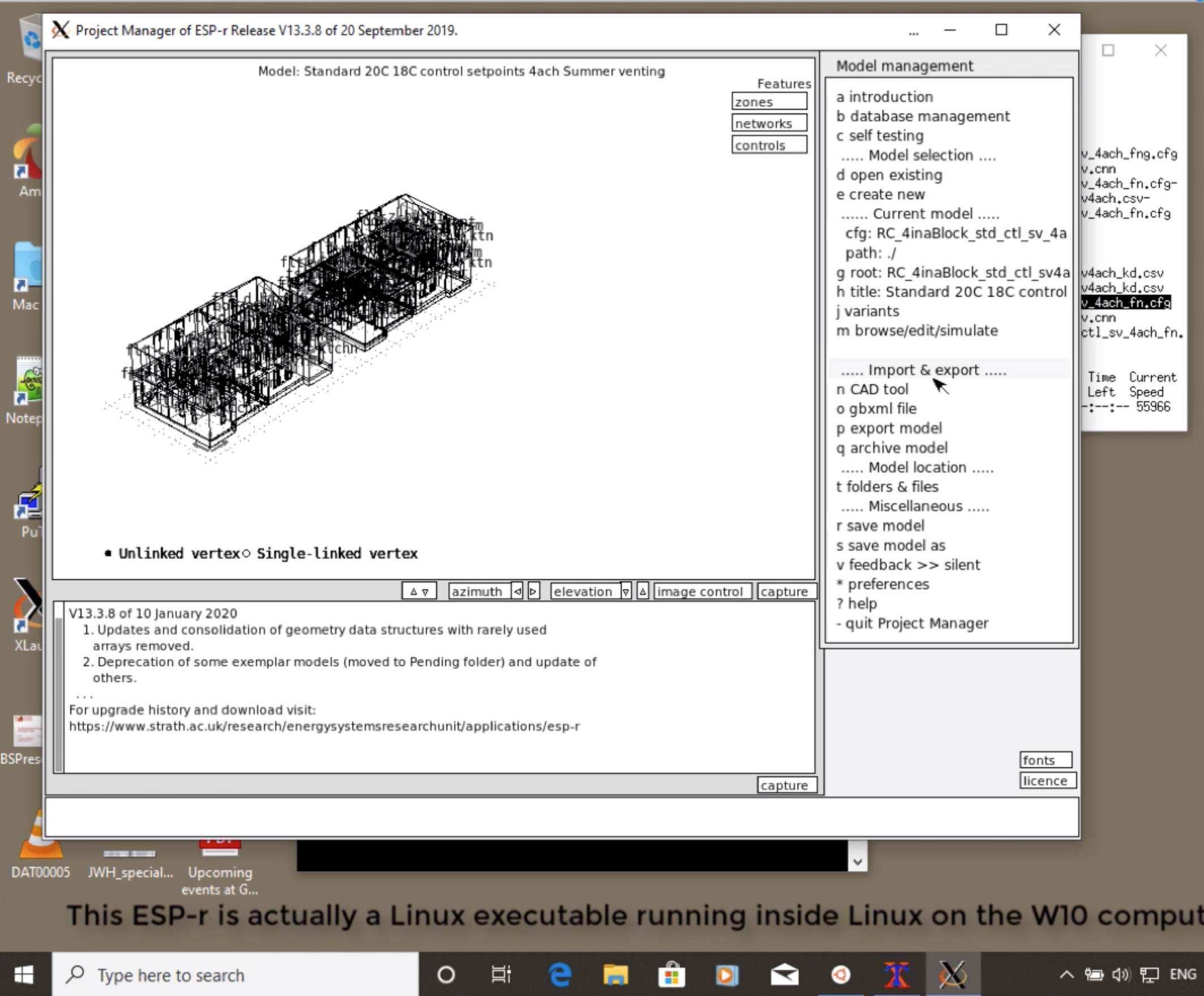
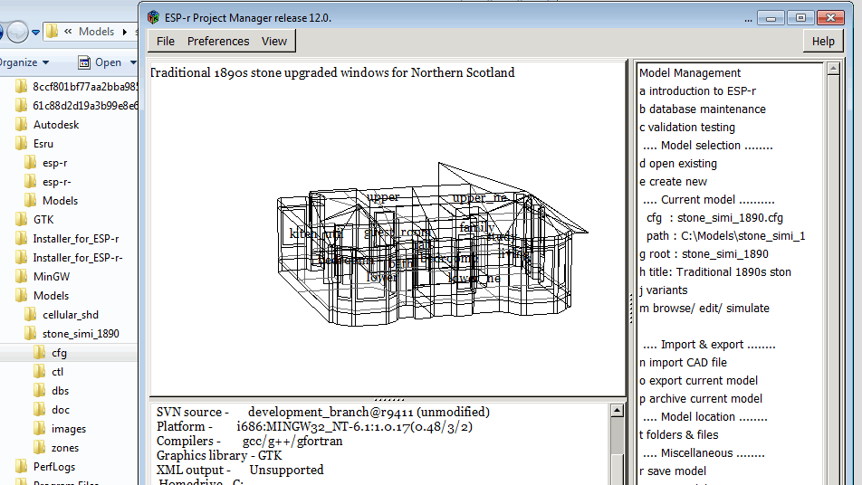
There are currently three interfaces for ESP‐r. The X11 interface has its roots in the world of UNIX and Linux. The cross-platform GTK graphic library version is primarily used for the Native Windows version. The third interface is a pure‐text interface (as seen below) which is intended for scripted production work or to enable ESP‐r to act as an engine for other software. Both the X11 and GTK interfaces will have essentially the same menu entries and the same initial key character so Figures often use the pure-text layout rather than a captured screen image.
 Standard data maintenance:
   Folder paths:
   Standard <std> = /opt/esru/esp‐r/databases
   Model <mod> = no model defined yet
  _______________________________
a annual weather        : <std>clm67
b multi‐year weather    : None
c material properties   : <std>material.db4.a
d optical properties    : <std>optics.db2
e constructions         : <std>multicon.db5
f active components     : <std>mscomp.db1
g event profiles        : <std>profiles.db2.a
h pressure coefficients : <std>pressc.db1
i plant components      : <std>plantc.db1
j mould isopleths       : <std>mould.db1
k CFC layers            : <std>CFClayers.db2.a
l predefined objects    : <std>/predefined.db1
  _______________________________
? help
‐ exit this menu
The Interface Appendix shows typical dialogues as well as a discussion of how to automate simulation tasks.
Exporing while reading
Strategies works better if you combine reading with doing. If you want to follow-along with the ESP-r Exercises check out Install Appendix for installation and first use hints on different operating systems.
Chapter 1 INTRODUCTION
Strategy is a high level plan to achieve one or more goals under conditions of uncertainty…and where the resources available to achieve these goals are usually limited. Wikipedia
Tactics are the actual means used to gain an objective/goal
Strategies for Deploying Virtual Representations of the Built Environment presents a mix of strategies and tactics for:
translating client questions into virtual representations that are are no more and no less complex than is required for the task
responding to what if questions and making models that are also fit to answer the next question the client will ask
discovering valuable patterns in the clutter of performance data
re‐discovering the power of pencil and paper planning
clearly observing what is to be simulated in order to capture its essential character.
round up the usual suspects from Casablanca (1942) and is the 32nd most used file quote Wikipedia
What you are reading is the antithesis of rounding up the usual suspects. It proceeds from the belief that there is both art and science in the design of the virtual worlds which exist within simulation tools. We choose what to include and we set the boundaries for numerical tools.
In this book the general purpose simulation suite ESP‐r is used as a platform for exploration (as in the aka ESP‐r Cookbook in the title). ESP‐r unashamedly defers to the user’s judgement for the level of abstraction and detail included in each analysis domain and thus is a fertile ground for the discussions which follow. In ESP‐r:
there are multiple approaches to most simulation tasks which the discussion and the accompanying exercises explore,
there are multiple solution domains and thus many of the complex interactions which can be observed and measured in the real world can also be explored,
functionality follows description and thus the discussion can explore a range of complexity from models created over a coffee break to those which can only be managed within the resources of well‐founded simulation groups,
and there are rich facilities to explore performance patterns.
And although users can coerce ESP‐r to use non‐dynamic representations, ESP‐r is also unashamedly a tool for the solution of dynamic thermophysical interactions within the built environment.
1.1 Virtual physics in the design process
The design process proceeds on the basis of the beliefs the design team holds about how the current design satisfies the needs of the client. Testing whether such beliefs are well founded is a classic use of simulation. The way we design such tests and our approaches to the use of numerical tools are core issues in the sections that follow.
For example, some design teams operate on the assumption that buildings are rarely comfortable without the intervention of mechanical systems. Are such assumptions true for a given design? Let’s use simulation to test how often a building works well enough to satisfy occupant requirements without such interventions and then explore options.
Many design methods focus only on extreme conditions. What is the cost of this? Let’s use simulation to explore the nature of the building’s response to transition season weather as well as diversity in use and, by understanding demand patterns, devise environmental control regimes which work well across a range of conditions.
Practitioners employ a variety of working practices. Unfortunately, some make excessive demands on staff and computational resources to the point where we fail to deliver on time, fail to notice opportunities or fail to identify risks inherent in designs. Practitioners have a choice - to be tool driven or attempt to drive-the-tool. Opinionated and productive practitioners tend towards the latter and hopefully the discussion and hints that follow will also allow you to drive-the-tool.
For simulation to do it quicker, cheaper and better guidance is needed. Reference handbooks such as the CIBSE AM‐11 include valuable discussions about working practices and procedures. A must‐have for any library and a rich resource for saving time and sanity.
Software vendors are a mixed resource. They often seem to believe their own hype about ease of deployment. And contextual help within tools, no matter how extensive, deals with a sub‐set of the skills needed to make informed decisions.
Learning how to use simulation tools tends to follow three paths ‐ the mentor path, the workshop path and the there‐be‐dragons path. Groups working with simulation often use a mentor‐based approach to increase skills and productivity but this is difficult to scale. Two or three days of initial workshop, with subsequent advanced workshops and occasional email support works well for some practitioners. In the absence of contact with mentors and workshops, practitioners are often confronted by the arbitrary conventions which are endemic in simulation tools. Each button press enters new territory ‐ thus the term there‐be‐dragons.
Working at the edge
The author has observed that users of simulation tools have ranges of model complexity within which they are comfortably productive and beyond which there is an increasing risk of fatigue and error. Most experts plan their work and their models to avoid the computational and complexity limits of their tools. A failure to constrain project complexity is a classic way to run short on options.
There are many possible vectors for this, some involve actions by the user and some can be gaps in the logic of the software. Caution and paranoia are useful attitudes:
Generate model contents reports as the model evolves and use visual comparison tools to confirm changes.
Automate the extraction of a range of performance metrics as the model evolves to identify unintended consequences as well as opportunities.
Involve colleagues as reality checkers of model design decisions as well as observers of performance changes.
Think. Before you press. OK.
Make frequent backups (create habitual triggers for invoking backups).
We invest in the creation of models in order to observe the performance of our designs. However, model complexity impacts the computational and staff resources associated with data mining. As performance data grows into the tens or hundreds of gigabytes disk access becomes problematic. However, the real limit is our ability to find patterns in such huge stores of information.
Entropy haunts parametric studies. So much can be invested in setting up a base case model that supports the anticipated design variants and reporting requirements. The whole edifice can be destroyed by demands to tweak the metrics to be captured or the form or composition of the base case.
Strategies focuses on how we might design our models as well as the nature of the assessments we commission and the metrics we seek to recover. Whether you are a solo practitioner or a member of a team, a clear recognition of limits is critical.
The discussion will also: - clarify the jargon used in the simulation community, - provide background for those who are delivering workshops or formal courses, - provide commentary on working practices for those who manage simulation teams. - inform your exploration of example models distributed with simulation suites whether they illustrate semantics and syntax, are derived from real projects and might be considered exemplars of best practice.
Abstract training models may not be representative of best practice, they may not scale well and may attract the attention of an attorney if used in a real project. Consulting or research derived models might push the limits of the tool in order to deliver specific performance information.
Exercises are used to illustrate the translation of simulation theory into specific working practices. Beyond the how of the keystrokes are hints about what to look for as well as decisions behind the approach. Well worth following. Strategies works better if you combine reading with doing. If you have not yet setup ESP-r on your computer see the Install Appendix.
In order to explore simulation you need a working folder on your computer for simulation models. Exercise 1.1 covers the steps needed for Linux, OSX and Windows.
1.2 An example of quicker, cheaper better
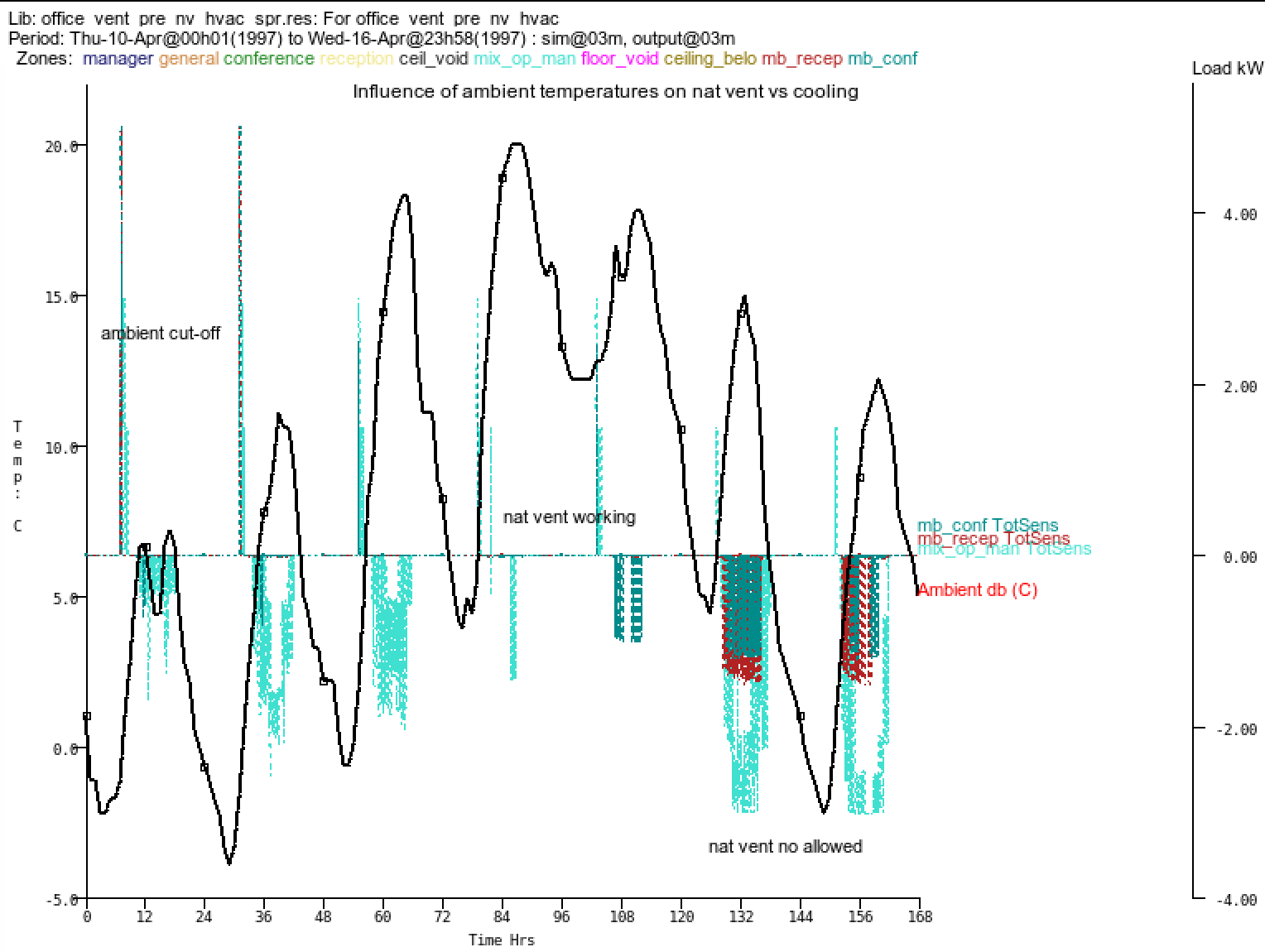
Back in the days when Intel Pentium 4 processors were becoming fashionable, the author had a project to evaluate whether mechanical dampers in a facade of an office building could be used as an alternative to mechanical ventilation during transition seasons.
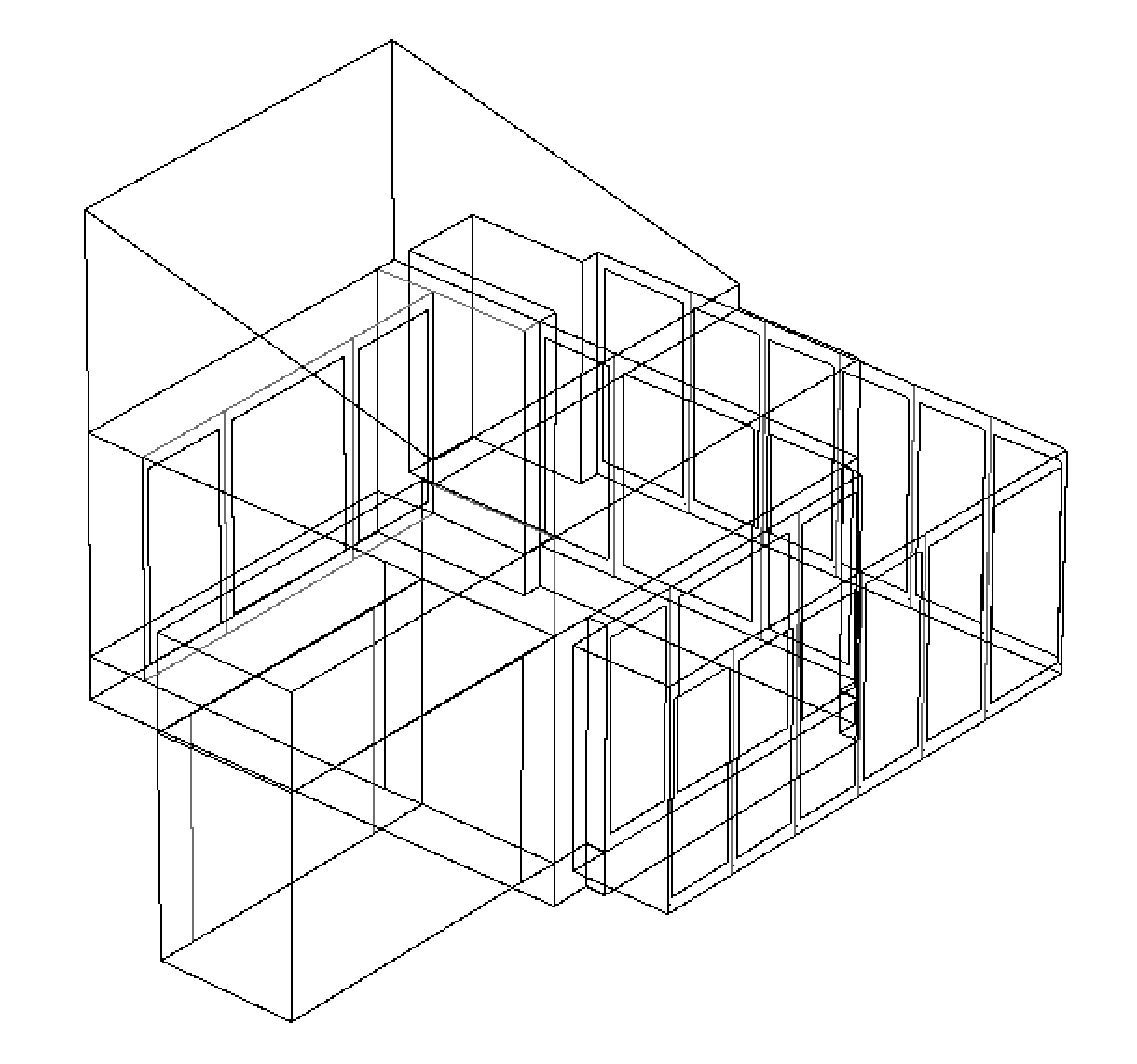
In order to assess the performance opportunities and risks of this hybrid scheme, a base‐case and three variants of the model in Figure 1.1 were created. It included explicit internal mass, facade elements and shading devices, as well as two variants of air flow network and three control schemes.
The model can be browsed from within the ESP‐r project manager in the real projects category of the training exemplars. Exercise 1.2 takes you through the steps of exploring this model.
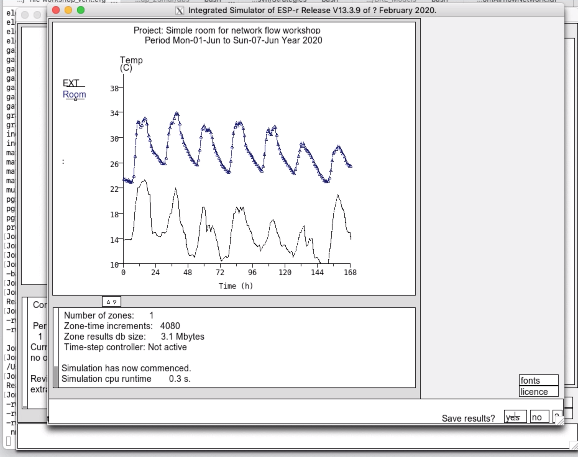
How long should a client expect to wait for feedback? In the event, a synopsis of the findings was available five hours after the plans and sections were first opened. Examples of its performance can be seen in Chapter 11 Figure 11.31.
To ensure the facade ventilation model contained no more and no less than was required to satisfy the brief the first hour and a half was devoted to planning the model:
establish the extent of the model and the likely nature of what‐if questions
review existing models which addressed similar issues
identify weather patterns which would clarify the building’s performance
review available constructions, identify additional items needed and possible variants
define the resolution of the model (form, composition, controls, schedules) required to answer performance questions
define the analysis resolution of the model (e.g. radiant exchange, air flow, systems)
plan model zoning, sketch the model, decide naming strategies and note critical co‐ordinates
sketch air flow paths and gather relevant data
outline room usage patterns, internal gains and environmental controls
plan the calibration tests to be carried out
review sketches and the approach with colleagues as a reality check
define the sequence of tasks needed to implement the model
begin documentation of the model and its assumptions.
Figure 1.1: Portion of an office building ‐ the five hour project
This sequence of planning steps has been used with scores of models. With minor tweaks it should be applicable to other simulation suites.
The model creation sequence: - populate materials and constructions databases - define the model calendar with day types needed for operational and control regimes - digitise the initial layout of the rooms and ceiling void - focus on managers office, adapt framing and glass in facade and passage and fully attribute surfaces - replace initial facade surfaces in other rooms with manager facade elements - create desks in the general office and then replicate/adapt to other spaces - adapt the ceiling void via copy/invert of ceiling surfaces in rooms below - use the topology checker to establish thermophysical links between rooms - generate a model contents file and do a quick scan for the usual QA suspects - carry out shading and insolation analysis for each of the zones with facades - calculate surface‐to‐surface view‐factors to support long‐wave heat transfers within rooms - define the operational characteristics of the managers office (including diversity) and then adapt for other zones - define a reality check imposed infiltration regime - define air flow networks ‐ initially with vents closed for calibration - define air flow controls ‐ a sticky open/close controller and a proportional opening controller - define assessment periods for winter‐cloudy, winter‐sunny, spring, summer‐cloudy, summer‐sunny weeks - update model contents report and invoke a one week assessment to confirm model syntax - explore model variability of air movement and risk of overheating or over-cooling via a typical week in each season.
This sequence of tasks is efficient in terms of creating the underlying data model as well as in the use of simulation facilities. It is pedantic where needed and ruthless in constraining the bounds of the problem. Users of other simulation suites will, of course, discover slightly different paths.
About one and a half hours was spent creating the model. There were a couple of typos in defining the schedules of internal gains that were identified in the model contents report. The model was accepted by the simulation engine on the initial pass.
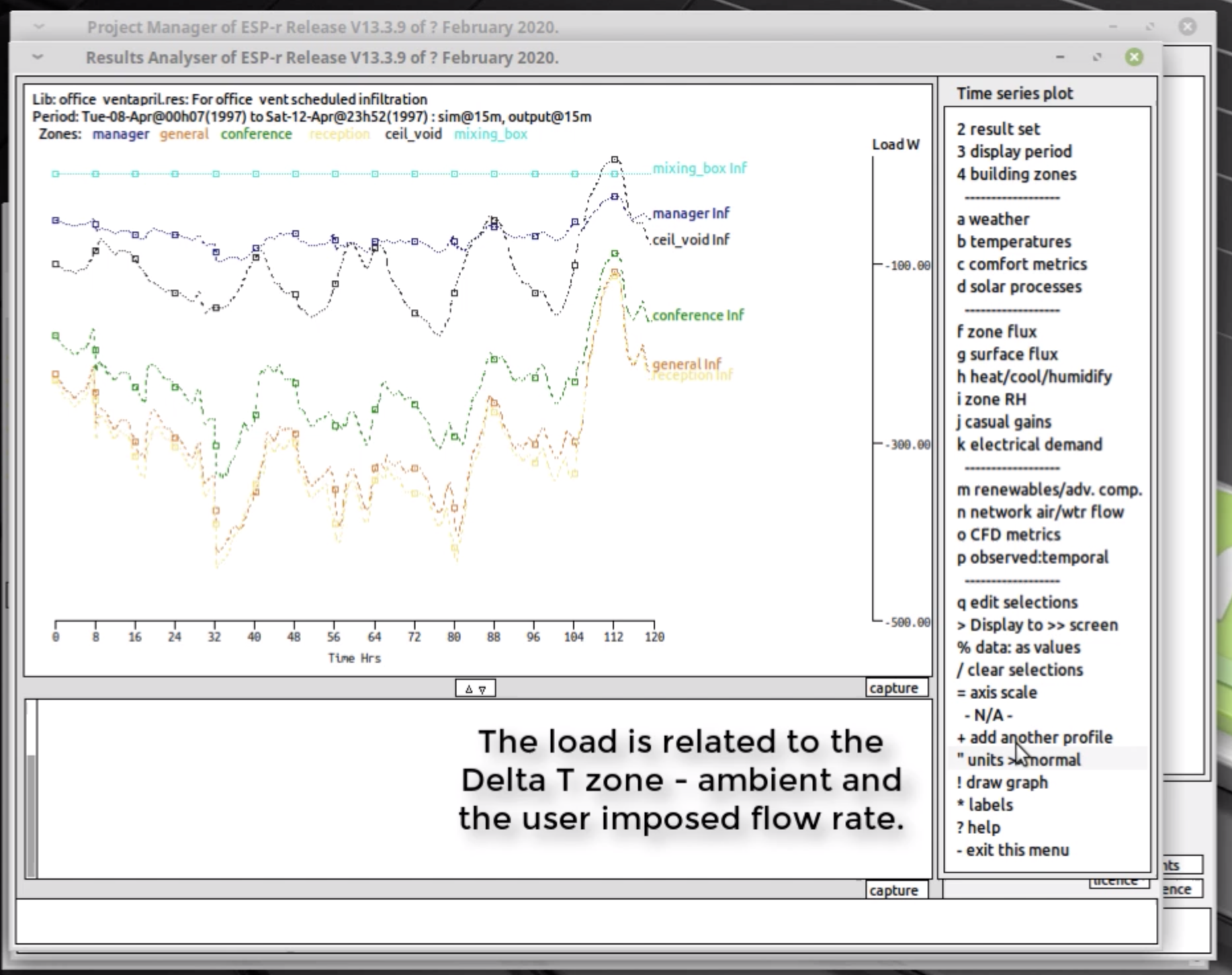
About a half hour was spent in calibration using the one week assessment periods identified in the planning stage. Calibration started with a reality check via fixed infiltration assumptions and was then compared with the infiltration‐via‐ flow variant. The second phase looked at patterns of differences in temperatures and loads from infiltration and inter-room air movements. The third phase incorporated damper controls. Again, checks were made over the range of weather conditions in the defined weeks and the controls tweaked.
The remaining time was living with the model in order to understand the conditions associated with beneficial use of the dampers as well as the risk of discomfort. Graphs and reports from interactive sessions were collected along with wire‐frame images of the model for inclusion in the report.
If we did that project today
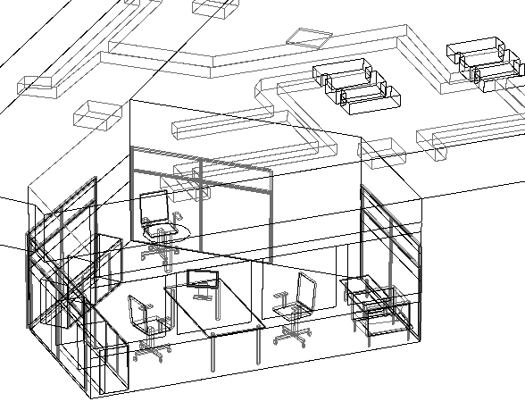
Tools and data models have evolved. Databases include provenance and most are now organised by categories. There is a library of common room use schedules with diversity. Model contents reports have evolved. There are libraries of pre-defined furniture, fittings and common building elements such as stairs which supports higher resolution. You can see a video of a session populating a computer room with desks and monitors. The scope and extent of uncertainties can now be formally described.
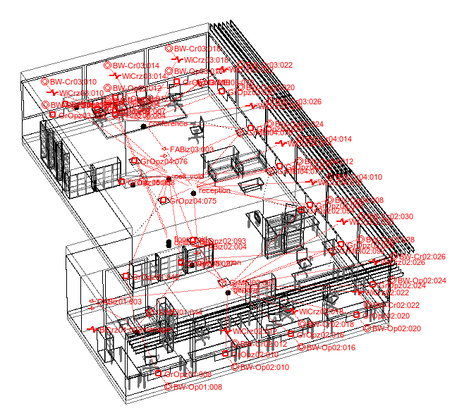
Figure 1.2 A high resolution section of an office.
For some practitioners a more important change has been in attitude to allowing the physics to be more robustly expressed. Imposing infiltration as if we were dieties, is so 1990s. Attributing the models as to where air might flow or where flow might be imposed or constrained and letting the tool create compute flows is the new normal. Changing attitudes toward levels of abstraction are also evident and Strategies will delve into this evolution as well.
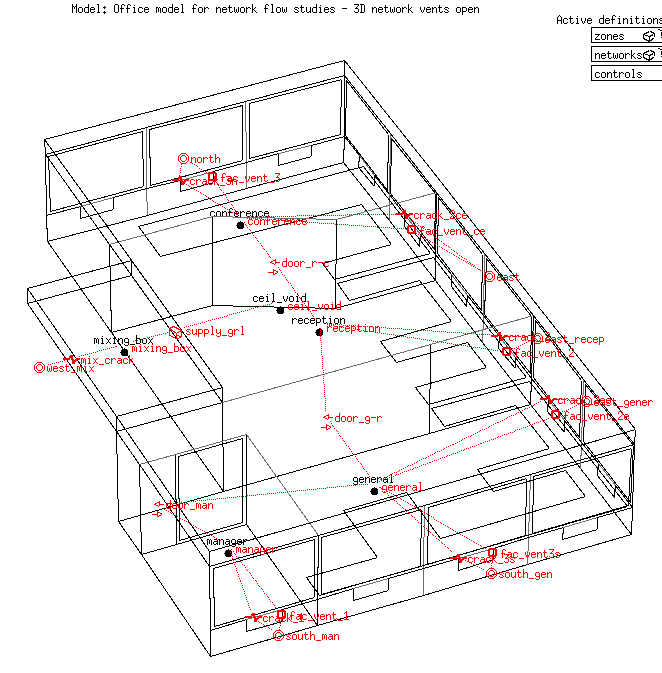
So within a similar time budget planning tasks could be streamlined. We could create a better model (such as seen in Figure 1.2). For example, we could increase the geometric resolution by using pre‐defined desks and select a diversified conference room occupancy pattern. We would attribute the model surfaces to identify the location of cracks and doors and inlet or extract grills and then check the overlay of the generated network to see if it matches out sketches. We could extend the scope of the enquiry to check the transition between natural and mechanical ventilation.
We would use the improved model QA facilities more frequently to identify glitches and more quickly produce an Appendix for the model contents to pass to our colleagues and the client. A modern computer would, of course, support a finer time resolution in the assessments as well as visual assessments via Radiance.
Check out the differences in the empty and fully populated versions of the office model via the latter portion of Exercise 1.2 Exercise 1.2.
In addition to browsing models we want to be able to return to a prior model and continue working. To explore options for working with existing models go to Exercise 1.3.
Other simulation suites will also have evolved and offer shiny new buttons to press. The point of Strategies is to decide for ourselves which of these will assist in delivering better information into the design process.
1.3 Questions we should be asking
Let’s turn to the strategy and tactics demonstrated in this project. Clients ask us questions ‐ but what are the questions we ask ourselves as we plan and create our virtual worlds?
Let’s expand on the nature of the planning decisions behind the above list. Being pedantic during the planning stage often speeds up subsequent tasks. In the left column are high level design questions and on the right is a translation into a simulation context.
Table 1.1 Initial questions
Design Question
Simulation Questions
What specifically do we want to know about the design?
What kinds of performance should be measured? Where should these measurements be taken? What signifies acceptable performance? What level(s) of model details does this imply?
Does the available information match the tool requirements?
What is the essence of the design in terms of form, composition, operation and control? What thermophysical interactions need to be represented? What tool facilities should be employed and what skills are required?
Is our approach robust?
Can I sketch my ideas for the model and explain my methodology? Are the project goals matched with staff skills and tool facilities? What would we do now to make it easier to work with this model again after a four month delay?
Are the performance predictions credible?
What assessments will help us gain confidence in the model? What diversity should be included in use and control? What is expected of a best practice design? Who else should review these performance predictions?
How might the design fail?
What boundary conditions and operating regimes might cause failure? What might be the unintended consequences of a design change?
What are the opportunities?
What would provide clues for improving the design? What change signifies improved performance? What is the next question the client will ask?
Without careful consideration of these questions we miss out on the value‐added aspects of simulation which cost little to implement but deliver substantial benefits. It is also an excellent filter for identifying aspects of a design that can be handled abstractly or omitted. More examples of design questions and actions can be found here.
1.3.1 What is fit for purpose?
The approach we take is dependant on the questions we wish to address with the model as well as the specifics of the data model and facilities offered by the simulation suite.
Lets look at some classic design questions:
general comfort and energy demands at peak and moderate weather conditions require only a moderate geometric resolution e.g. correct volume of the space, approximate location of doors and windows
comfort at a specific location requires higher geometric and thermophysical resolution, especially if temperatures are likely to be vary across a surface
environmental control what-ifs require the response characteristics of the building and environmental controls are reflected in the model as well as in assessment timesteps
projects involving comparison of predictions and measurements require a pedantic approach to match the description, operation, and controls within the virtual and physical realms
visual comfort will require higher geometric resolution for facades as well as furniture and outside obstructions
distribution of air temperature within a physical space may require that it be represented by more than one thermal zone or that it include a computational fluid dynamics (CFD) domain
For example, a passive solar design will be sensitive to heat stored in the fabric of the room, details of glazing in the facade as well as heat and mass transfers to adjacent rooms. The surface temperatures in a sun patch might be elevated. To find out where the sun falls in the room at different times of the year we might create a rough model and then check what we can see in a wire‐frame view at different times of the year. Our goal would be to find out if we need to subdivide surfaces to better reflect the temperature differences in insolated and un‐insolated portions. We can then make a variant of the zone with higher geometric resolution and compare the predicted surface temperatures.
1.4 Responding to the client specification
Simulation models have a context within which they are created and evolve. In a design project the client’s specification and design questions form the context. In the office building in the previous section, a portion of one floor of the building provided sufficient context for project questions. The zoning allowed for differences in the resulting temperatures to be tracked.
Consider what simulation looks like from the clients perspective and choose, if possible, design the model to limit their confusion. Planning decisions can influence the resources needed by others to understand both the intent and the composition of models. Some models tell a good story allowing design teams and clients to move on to substantive issues. Other decisions result in models with impose a considerable burden on the design team, puzzled expressions when clients view the model. Making clients work hard is a questionable business strategy.
Ideally we design models to be no more and no less complex that is required to answer the clients design questions. If we are clever our model will also be designed to answer the next question the client will ask. A model which is overly simple may fail to represent the thermophysical nature of the design. A model which is overly complex absorbs resources which may not be sustainable.
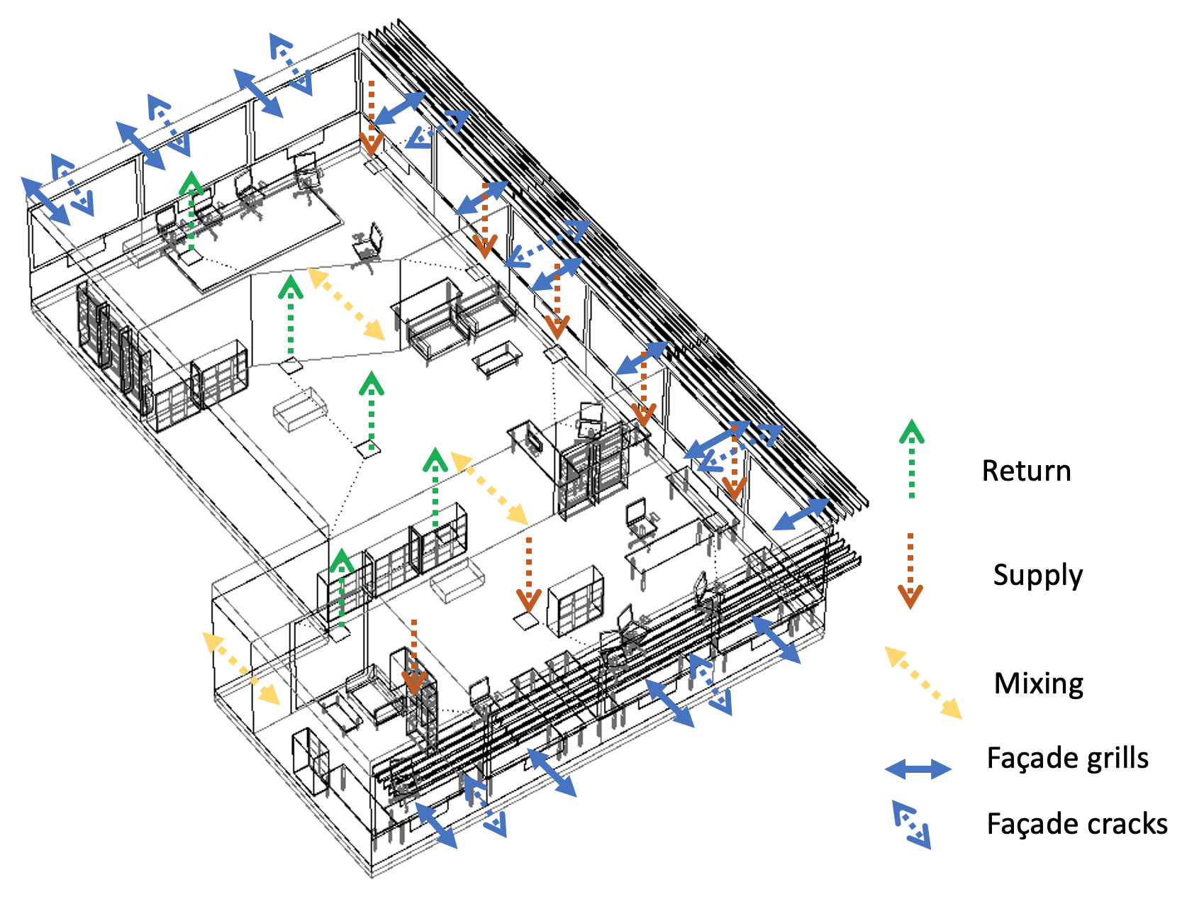
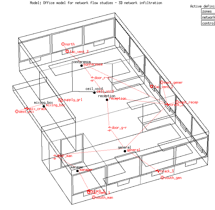
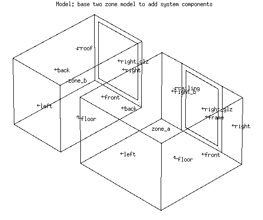
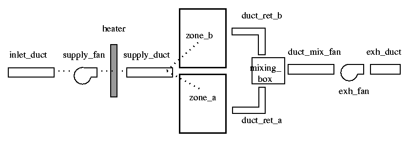
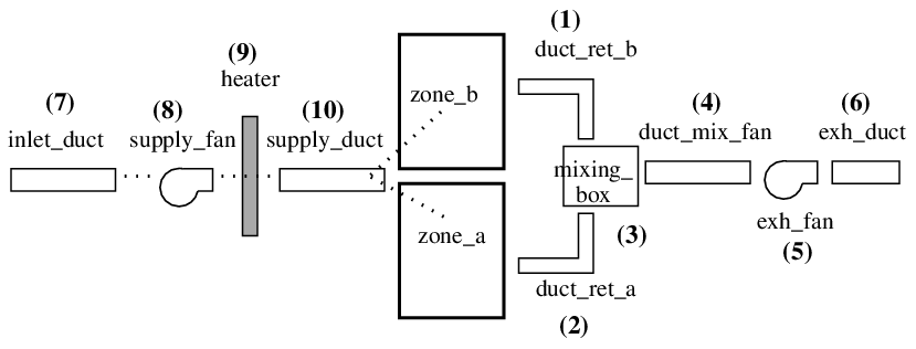
Thus, the office model also included a suspended ceiling zone because it was likely to be at a different temperature from the occupied space (lighting was embedded in the ceiling). The inclusion of desks at the perimeter provided visual clues for the client as well as ensuring that overheating from solar gains near the facade are accounted for. The mixing box was included for a possible subsequent assessment of hybrid ventilation.
Tactically:
it was quicker to include entities in the initial model than to retrofit
it made the wire‐frame view of the model self‐explanatory so that the focus of the reporting could be about the performance rather than geometric abstraction
starting with a infiltration-focused flow network variant helped prove the network, provided early indicators of facade sensitivity as well as the temperature driven flow between spaces prior to invoking the dampers.
Focusing initially on a portion of a building is a powerful approach. Experts often generate focused models that evolve quickly and are then discarded once the question of the moment is dealt with.
In a research project the goals of the project are no less critical to planning and implementation of tasks. The following table illustrates planning stage issues:
Table 1.2
Core issue
Related issue
Actions
Does the client/design team have prior experience with simulation?
Experience eases the educational task and tempers client expectations.
Ensure time and resources for briefing the client on the information they will be asked to provide.
Does the client/design team know what performance data and reporting can be generated?
Management of expectations and selection of reporting format(s).
Review client preferences and clarify potential misunderstandings in deliverables.
Has the client expressed beliefs about the design’s performance?
Create focused models to test these beliefs.
Confirm if typical performance data for the type of building is available as a reality check.
Has the client indicated what criteria would signal success or failure?
What are likely modes of failure? What needs to be measured to identify risk?
Confirm that the tool and staff can support such assessments?
Is the project dealing with a range of issues?
Do we require several models or model variants.
Define working procedures and staffing requirements.
Are what-if questions general or product specific?
Is the role of the simulation team reactive or proactive?
Are supplied specifications appropriate and in the clients interest?
Do what-if questions pose parametric questions (e.g. which skyight area between 12 & 36% is the point where cooling demand escalates)?
Is it possible to automate parametric excursions?
Manually check 12% and 36% options to establish sensitivity prior to implementation.
Have we done something like this before?
What did we learn in the previous project? What proved to be difficult?
If we adapt & evolve how does this impact procedures and staff resources.
A potential project will be discussed with a client in a meeting tomorrow.
Who should take part? What key phrases are important to listen for? How much do we need this project?
Review details of similar projects. Review bidding criteria. Ensure that presentations and sample reports are available if needed.
Each core issue can be expanded to more specific tasks during the planning phase. Over time these can form the basis for procedures and checklists.
1.5 Model entities
The art of creating models fit for purpose draws on our ability to select appropriate entities from within the simulation tool. Each entity has rules‐of‐use, descriptive and/or operational attributes and takes part in specific thermophysical interactions within the solution process.
What should be a straightforward task is complicated by:
poor observational skills (when surveying spaces we wish wish to model),
limited skills in reading construction documents,
omissions and obfuscations in construction documents,
a lack of insight into the underlying physics within elements of buildings,
jargon in the tool interface and supporting documents,
beliefs that the tool will shout at us if we do something stupid.
To illustrate some of these rules and attributes lets focus on a subset of definitions from the ESP-r Entity Appendix:
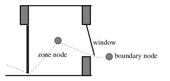
A thermal zone represents a volume of air at a uniform temperature and which is fully bounded by surfaces (see below). Within the complexity constraints of ESP‐r a zone can take any arbitrary form. A thermal zone might represent the casing of a thermostat, a portion of a physical room or a collection of physical rooms depending on the requirements of the project and the opinions of the user.
Within a thermal zone there is an air‐node energy balance. Air movement with the outside and with other zones in the model is included in this energy balance. Casual gains from occupants, lights and small power are also included.
A CFD domain can be associated with a thermal zone and/or mass flow nodes can also be associated with a thermal zone.
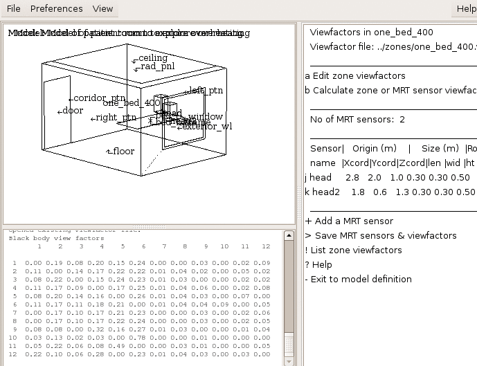
Long wave radiant exchange is supported between all zone surfaces. The default treatment is weighted by area and emissivity and the mrt utility is able to calculate explicit view‐factors for thermal zones of arbitrary complexity.
Direct and diffuse solar radiation is tracked within a zone. The default treatment is diffuse distribution of solar radiation entering the zone from the outside or adjacent spaces. The ish utility is able to calculate shading patterns on the facade as well as insolation patterns within a thermal zone of arbitrary complexity, including explicit internal mass represented via surfaces.
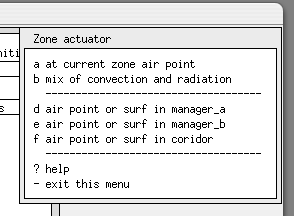
Ideal environmental controls can sense and actuate at the zone air node. Sensors can reflect the current air temperature or a mix of air and MRT. Actuation can be a convective injection at the air node or a mix of convection and radiation to be absorbed in the zone surfaces on an area/emissivity basis.
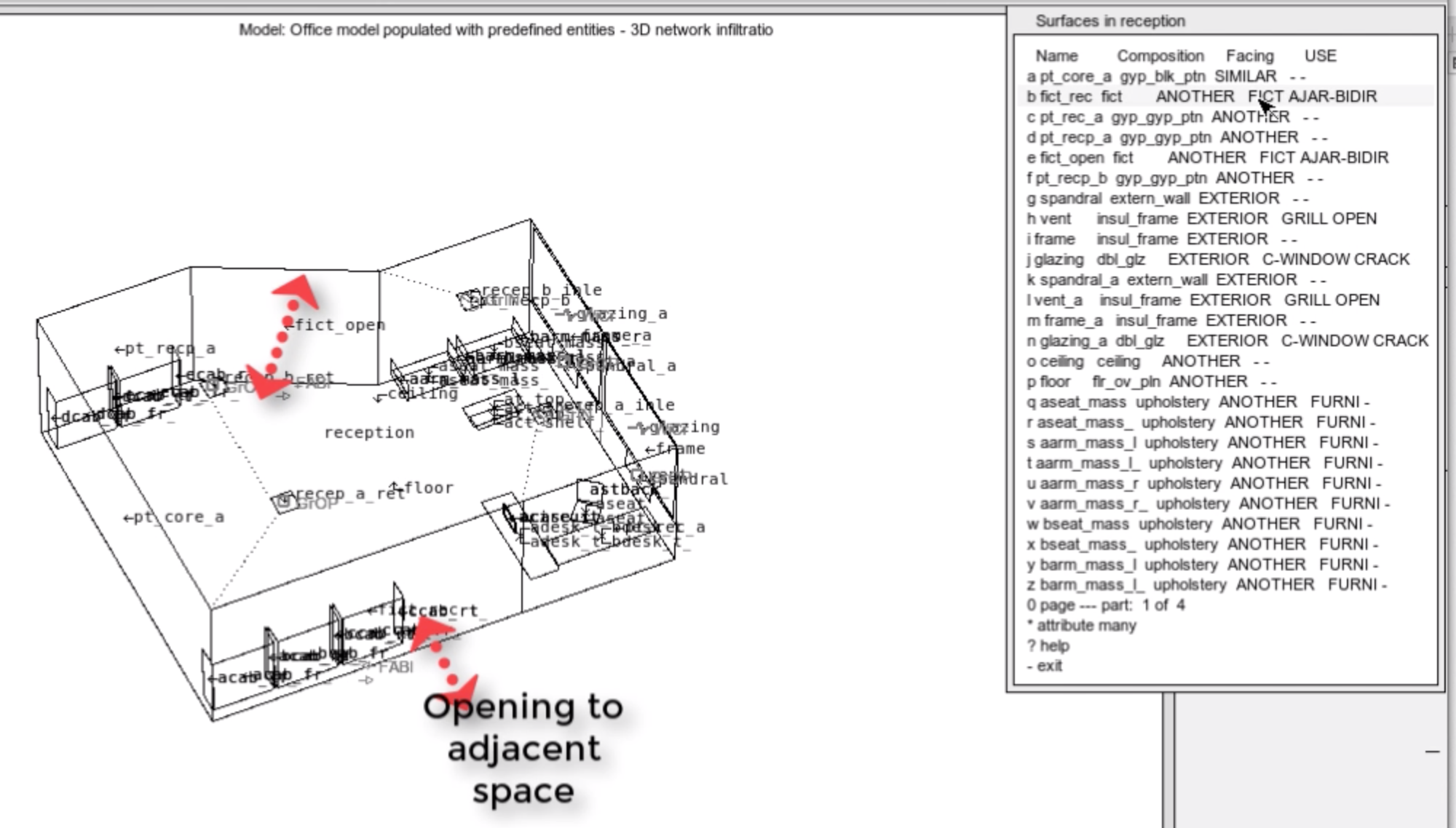
As zones must be fully bounded by polygons, openings between thermal zones must also be represented by surfaces (typically composed of a construction which minimally restricts heat flow). Air movement (mixing) associated with such openings is a separate definition in ESP‐r e.g. a scheduled zone ventilation or via cracks and bi‐directional flow components within a mass flow network.
A surface is a polygon composed of vertices and edges with attributes of name, boundary condition, thermophysical composition, optical properties and use. Within the limits of complexity a surface polygon can be of arbitrary shape as long as it is flat. A polygon can wrap around one or more child surface polygons.
During assessments a surface energy balance is maintained at the inner face and other‐side face of each surface. Each has a single temperature at any moment in time and the surface energy balance is consistent across each face.
For purposes of control, a sensor can be located at the face or within the construction or it can be the point of control actuation (e.g. an embedded pipe). Radiant heat injected into the zone via an environmental control is part of the energy balance of the surface.
One face is in contact with the zone air volume and it also participates in long‐wave and short‐wave radiant exchanges with other surfaces in the zone. Short‐wave diffuse radiation may pass to and from adjacent rooms. Convective heat transfer is evaluated at each time step and can optionally follow specific correlations or values derived at that time step from the CFD solution.
Surfaces have a boundary condition attribute specifies the nature of thermophysical interactions at the other face of the surface (see Entities Appendix).
Part of the chaos of working with multiple simulation tools is the diversity of entities and the subtle and not-so-subtle differences between the data models of simulation suiltes. It takes time to digest the documentation that is distributed with tools - for example, the EnergyPlus Reference volumes extend well past one thousand pages!
Check out the extended list in the Entity Appendix. And if you are using another tool consider how you would find such information in that ecosystem.
1.6 Model planning rules
Lets drill down into the design of simulation models in order to match skills, project goals and resources. Planning is a key step in exerting control over our numerical tools.
As a general rule, the volume of the air in rooms as well as the surface areas of facades, internal partitions and floors should be captured. We also want the mass within the rooms and within constructions to be appropriately distributed. This may or may not be straightforward to accomplish. Consider:
The scale of the building ‐ a residence might be abstracted so that each room is explicitly represented and the surfaces bounding the rooms and facade elements are located correctly in space. If this was attempted in a larger buildings with complex facades and scores of rooms, the model might exceed the available skill sets and resources. A degree of abstraction may be needed.
The regularity of the plan. Non-repeating patterns and non-orthogonal layouts are not easily to fit within an fixed gridding regime. Curving walls or facade elements will, of course, need to be subdivided into flat surfaces.
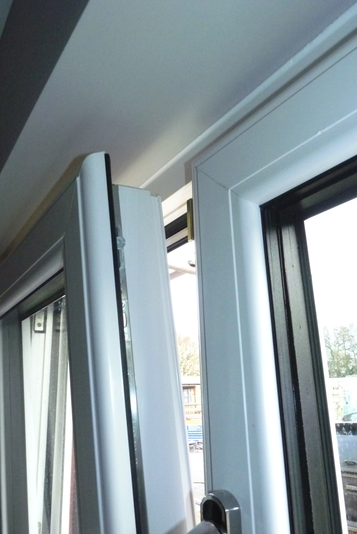
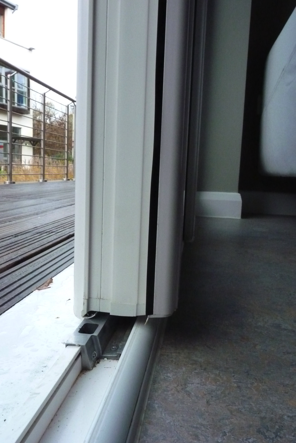
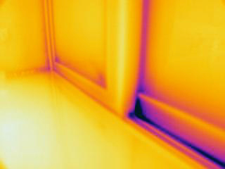
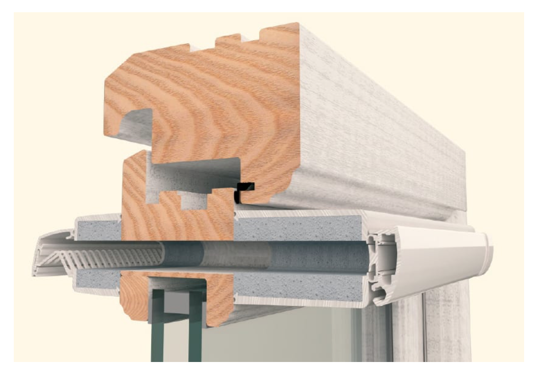
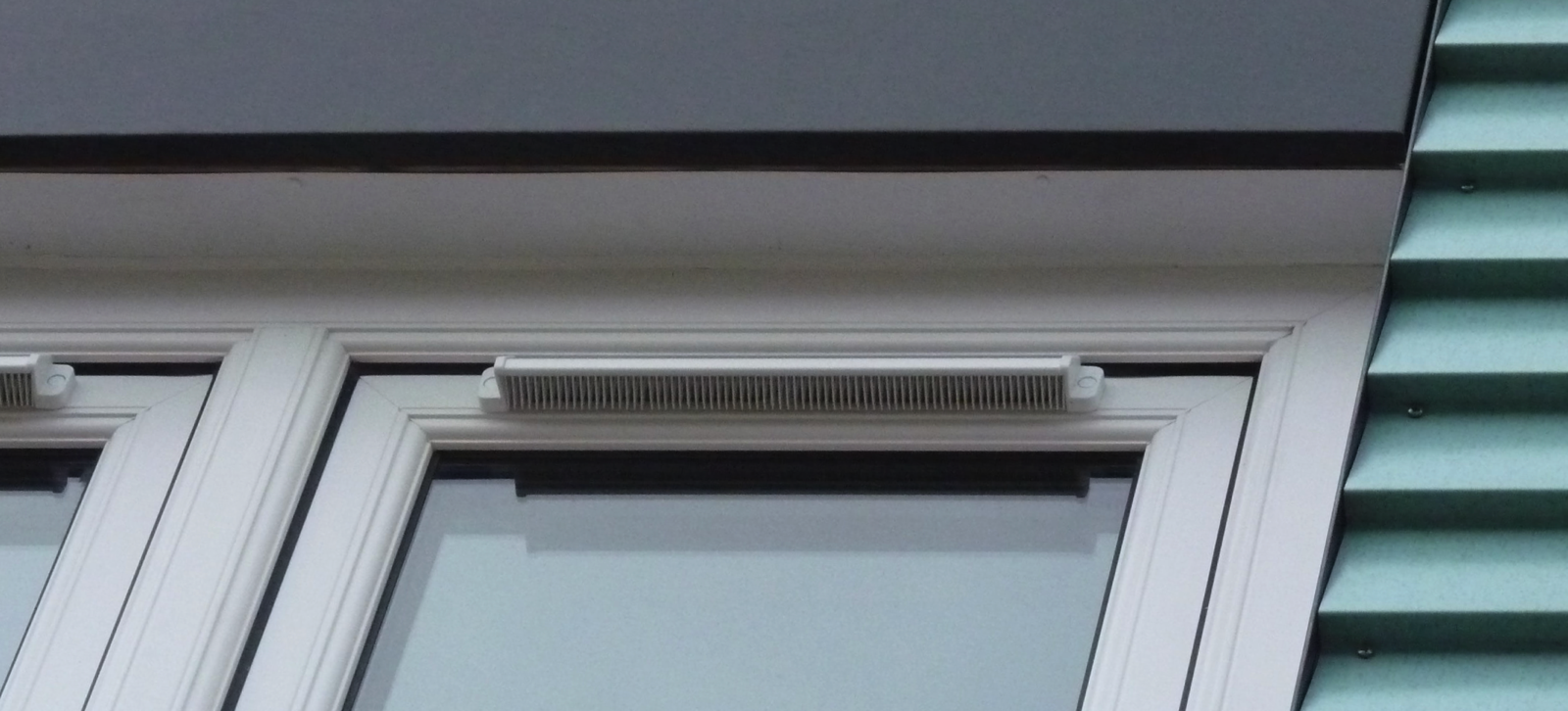
For many simulation tools the elephant in the room is the depth of facades found not only in traditional buildings but modern buildings with deep framing elements.
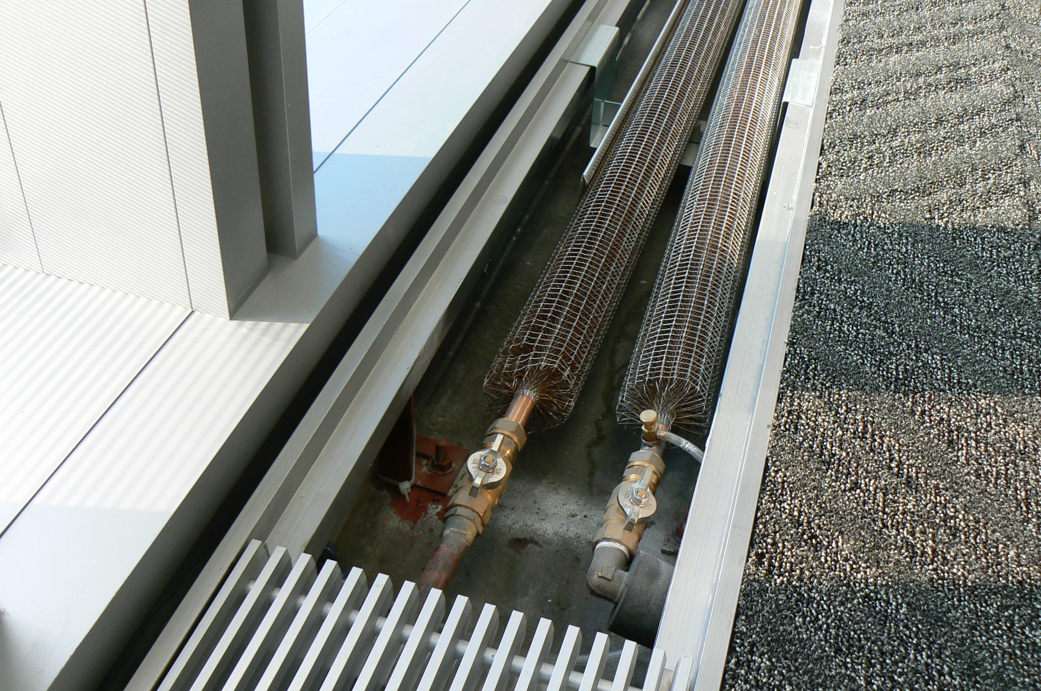
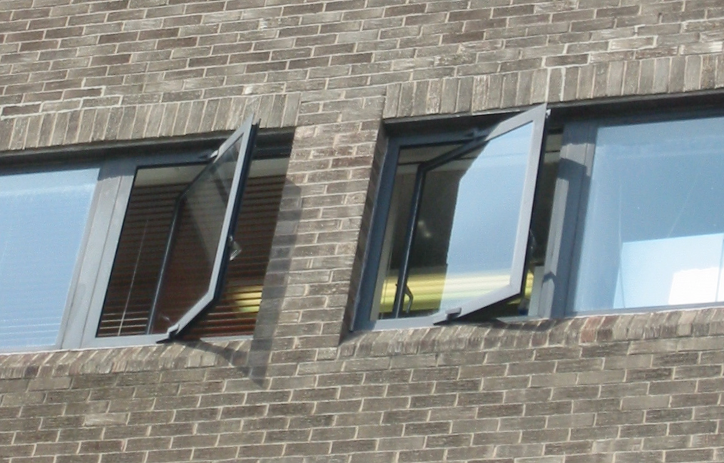
Mixes of fixed and operable elements within facades can host a variety of thermal bridges, air leakage paths and non‐uniform thermal properties. Far to often framing approaches 50% of the rough opening area and there can be a considerable difference between the inside and outside surface area of framing. It is difficult to justify 1D heat transfer representations in the images below.
Figure 1.3 Facade details that impact model planning.
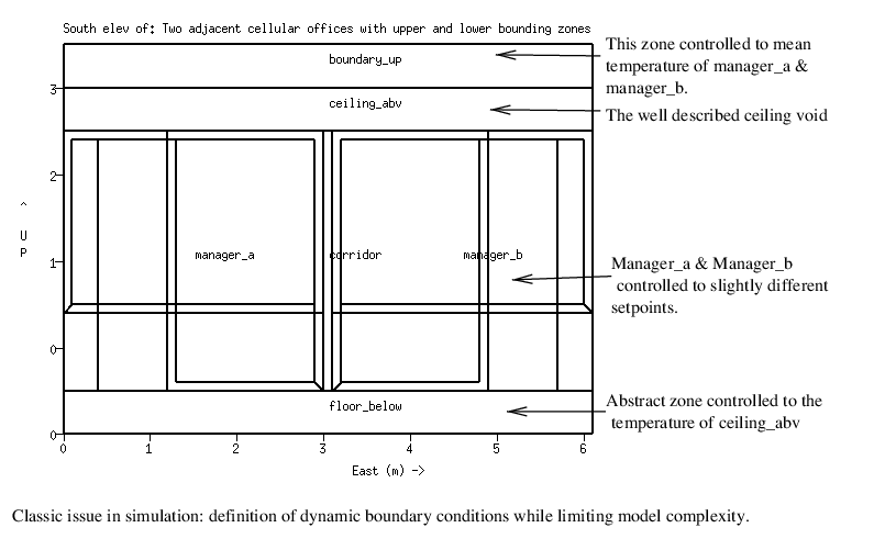
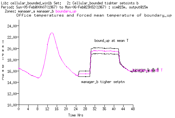
The existance of ceiling voids or raised structural floors. If there is little or no air movement these are often represented as layers of air in constructions. Where air movement is likely, temperatures are expected to differ, or there are heat gains within the void they may be better represented as separate thermal zones.
The thickness of intermediate floors. As ceiling‐to‐floor distances increase it makes sense to take height co‐ordinates literally.
The quality of the source drawing/images/CAD file has an influence on how we proceed. At one extreme there may be no construction documents. Sketches from a site visit may form the basis of the model. Documents may be archival hard copy and will need to be manually digitized.
And much that is included in CAD drawings is simply noise in the thermal domain. A client presented with a simulation model of fifty thousand surfaces or were told a box represented the Guggenheim in Bilbao would have equal right to demand an explnation.
The level of thermophysical clutter - architraves, window opening hardware, skirting boards and wiring chases. If the source includes one or two magnitudes of polygons than are actually required what filters are available? Would visual filtering while discritizing an image be more appropriate?
Some clutter may be useful to represent. For example, most buildings include furniture and fittings which can alter the response characteristics of the building as well as our perception of local comfort. Planning needs to consider their inclusion.
1.6.1 Discritizing designs
A typical approach is to use centre‐of‐partition and inside‐face‐of‐facades. However, for structural walls this can be problematic. And what about the ubiquitious but largely forgotten spaces such as wardrobes and cleaners closets which might not be worth explicitly representing but which impenge on the treated floor areas and air volumes we are interested in? What about service voids, raised floors and ceiling voids which might be at a different temperature?
Such questions apply irregardless of the form of the construction documents (CAD, archival hard‐copy, site visit sketches). Lets use a scan from an archival document of a 1961 tower block to explore such decision points.
Figure 1.4: Review of archival building plan
Most internal walls are ~100mm thick and choosing center‐line vs wall face will have a limited impact on the volume of rooms or surface areas. The structure between apartments is, however, ~200‐250mm thick. A compromise is to use centre‐line for the thin partitions and face‐of‐wall for the structure.
There are a number of vertical service voids. Ignoring them impacts zone vol‐ ume and floor area and it is likely that voids are rather different in temperature. The approach taken is to represent the walls but set them to a [similar] boundary condition. There are a number of small spaces marked [w.] and [c.] which are also treated this way.
However, there are linen cupboards which tend to be 1‐2 °C warmer than adajacent rooms and their walls set as [similar +2 deC] boundary conditions. The figure below shows how these spaces were adapted during the discritisation.
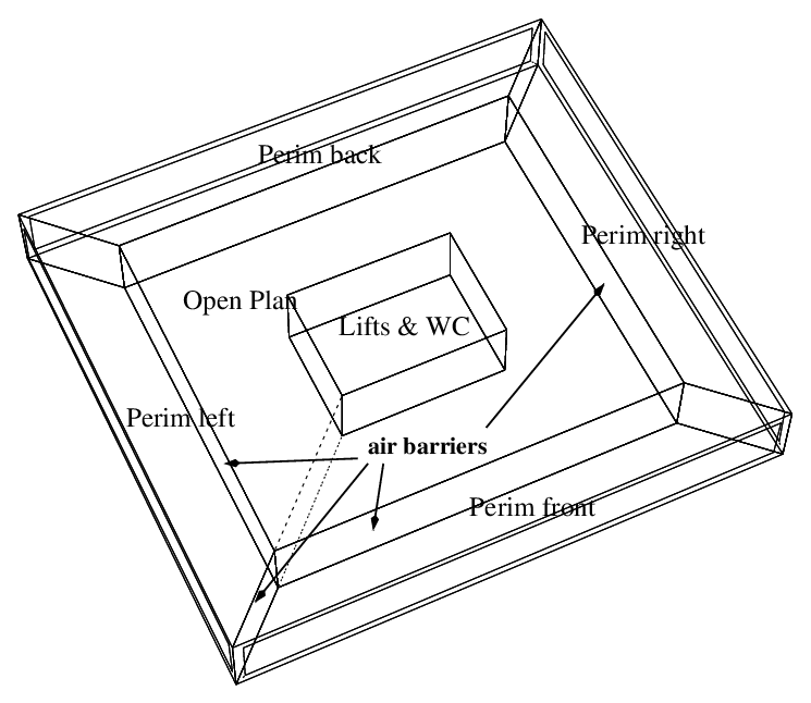
The access gallery are naturally ventilated spaces which act as a minor buffer to ambient conditions. They need to be represented by thermal zones so as to reduce the solar radition and wind exposure of the adjacent rooms.
Figure 1.5: Translating plans into model entities
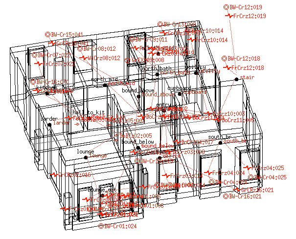
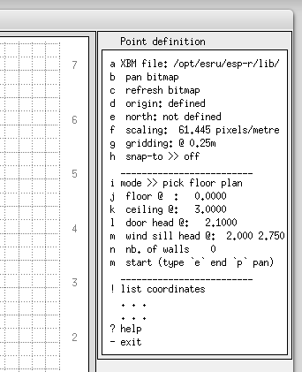
The initial model form which was derived from ESP‐r’s in‐built click‐on‐bitmap facility (explored in Seciton 2.8.2) is shown below. There are 42 thermal zones and ~640 surfaces to represent one level of the building. To complete the model geometry the rough openings in the facade need to have frames inserted (the frame area approaches 50% so is difficult to ignore). The stair zones could be adapted to expand over several floors as could the lifts.
Zones such as the drying area behind the lifts are well ventilated and thus form an important boundary condition for adjacent rooms. And there are 14 other drying rooms in the building so the initial polygons could be replicated above and below to form a single tall zone with suitable internal mass to represent the intermediate floors.
Figure 1.6: Resulting initial model
Another approach is to adopt a face‐of‐wall regime when creating a model. This implies explicit architraves. In smaller models this presents a minimal burden (in the order of minutes) for data input as well as a few seconds for assessments. The model shown in Figure 1.6 was created from site sketches drawn on graph paper assuming a 100mm grid and then scanned to underly the input grid in the interface.
Figure 1.7: Model creation following a face‐of‐wall regime.
In ESP‐r the boundary condition directive which specifies the thermophysical connection across a partition may be applied whether we use the centre-line approach or the face-of-wall approach. ESP‐r includes facilities to automatically discover that surfaces in adjacent zones likely represent faces of a partition or of internal mass and ask for confirmation from the user. Chapters 3 & 4 includes a number of examples of how building coordinates are treated in ESP‐r models.
Wire‐frame displays of zones and buildings in simulation tools often present facades as having little or no thickness. This fiction becomes problematic with high performance facades as well as traditional masonry construction.
Consider the modern office construction in Figure 1.7 (left) where there will be little or no change in predictions whether the centre line or the actual coordinates‐in‐space are used. However, when confronted with complex sections, such as seen in Figure 1.7 (right), simulation practitioners often resort to abstraction to capture the overall heat transfer.
How do we derive an appropriate abstraction when there are raised floors, ceiling voids, fan coil cabinets and spandrel sections? The latter are topologically solar collectors, and can easily reach over 60°C — a far higher delta T for the facade section at the ceiling void than most designers would expect. There are also thermal bridges at the spandrel to complicate matters.
Figure 1.8 Plan of a modern building and section at spandrel.
At the other extreme, historical buildings such as in Figure 1.8, can have deep facades which influence both the distribution of heat and light as well as partitions which vary in thickness. Essentially in most simulation suites we are approximating 3D heat flows via a collection of surfaces, each with a bespoke composition. The result, shown in the lower portion of Figure 1.8, substantially retains the volume and positions of the spaces rather than the exterior form of the building.
Figure 1.9 Plan and composition of a historic building.
Consideration also needs to be given to tolerances in dimensioning:
Would patterns of temperature and heating change if the volume of the space was off by the thickness of the wall?
Would more sunlight enter the room if a window was lowered by 5cm or the framing was accurately rendered in space?
Is it necessary to include furniture?
Our concern is to ensure that such descriptive decisions are unlikely to change performance predictions sufficiently to influence design decisions. Each of the above bullet points could, in fact, be tested by creating variant model and then looking at the performance differences between each approach.
An alternative is to formally describe what is uncertain in the model (e.g. the thickness of insulation in constructions, the density of concrete blocks, the magnitude of equipment gains, the arrival time of occupants, setpoint in thermostats, intensity of wind speeds etc.) and the scope of the uncertainty (e.g. which constructions, zones, control laws or which time period weather differs) and then comission Monti‐Carlo, Factorial or Differential assessments and have ESP‐r’s res module process the sets of predictions. This is discussed further in Section 11.6.
A further discussion about options for interpreting complex three dimensional designs and commercial facade sections into appropriate models can be found in Chapter 4.
1.7 Model composition
The planning process also includes consideration of the composition of walls, floors, roofs and facade elements. Simulation tools include named constructions which are made up of an ordered list of materials (each with a set of thermophysical attributes). Although each simulation suite has its own implementation, at the planning stage the issues confronting users are largely generic:
Identification of existing entities which are appropriate for the age and type of building.
Confirming that the attributes of entities are consistent with the construction documents.
Setting up place‐holders for aspects of the building which have not yet been decided.
Identifying alternatives for possible what‐if questions which may arrise.
Simulation tools are usually distributed with common data files for materials, constructions, optical properties and other entities referenced within simulation models. These are described in Chapter 3. The management of common data files is discussed in Chapter 14.
Some vendors invest considerable time and attention populating these resources. And what is on offer will have caveats: - entities may be regionally specific - entities may be idealised i.e. based on typical values - the provenance of entities may not stand up to close scrutiny - individual attributes may be at variance - is it close enough?
Whatever the tool’s facilities, we inevitably find that some entities we can copy and adapt and new entities to be added. Issues of provenance, corruption of common data stores and errors during data entry are critical.
Interpreting construction drawings can be a here be dragons task. Design teams create building sections for any number of purposes e.g. to record contractional decisions, to provide guidance on site, to assist bidding / costing / procurement. Design teams may know the key words they need to include for building compliance tasks but are less likely to be clear or consistant in documenting thermophysical attributes. Figure 1.8a demonstrates several issues:
They may or may not include product names (that shifts attention to the manufacturers site for what may be an interminable search for relevant information).
Notes such as or equal approved to give an overall floor U value of 0.15 W/m2/K is only one tangent we need to explore because the specifics of the screed or the block and beam system are unstated and there are a range of products allowed at the firewall.
And the design teams choice of where to cut sections may leave a number of junctions undocumented. The conventional fiction of typical sections i.e. with studs at 600mm centres is also a here be dragons trap. The actual details implemented on-site are likely to be far more complex and exceptions legion. The timber fraction which comes out of the factory is a late deliverable to the design process. An extreme example can be seen in lower portion of Figure 1.8a which includes a world-class collection of thermal bridges.
Figure 1.10 Incomplete sections and thermal bridge exceptions.
Jargon and convention also get in the way. Specifications often include un-real notations such as U-values. In some regions walls which include a so-called rain-screen use a convention to calculate this which strips off the outer layer and pretends the outside is as calm as the air in the room. This is not equivalent to how simulation treats heat transfer in walls.
Thus, practitioners often find it difficult to find a good match between construction specifications and vendor provided entities. Just as design teams can leave gaps in their specifications, simulation staff rarely appreciate the innumerable exceptions which may require the generation of alternative constructions as well as subdivision of surfaces to accommodate the exceptions.
Working through an example
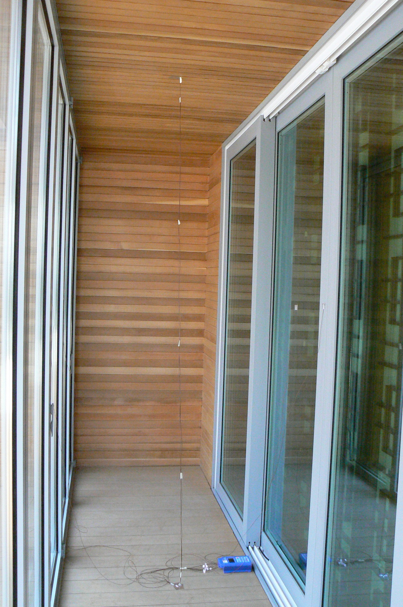
How might we represent the thermal performance of a 500mm thick masonry Trombe‐Michel wall so that it’s interactions with solar radiation, air flows and cross sectional temperatures are properly captured. Figure 1.9 is one approach with the stacked zones of the front facade air space where air flow is based on a dynamic solution (or perhaps a CFD domain). If you want to find out more look for the trombe_wall example models ‐ there are several variants with and without control of the dampers between the front facade and the office.
Figure 1.11 Explicit Trombe‐Michel Wall and temperatures.
As building facades adapt for ever higher performance thermal bridges also become an issue — this is discussed in Chapter 4. These can be approximated in ESP‐r via linear thermal bridges, but such entities require additional information which must be sourced from 3rd party software (see Figure 1.10) and translated into the syntax of ESP‐r.
Figure 1.12 Thermal bridge effects at a corner.
Most simulation tools default to one dimensional (1D) heat transfer within constructions with homogeneous and/or nonhomogeneous layers. ESP‐r offers this, but the greater challenge is that many building junctions are not well represented by 1D heat transfer. Although ESP‐r can solve 2D and 3D heat conduction the information requirements are daunting and are not discussed here.
1.8 How buildings are used
If we modelled a library and did not include some representation of the book collection we would need to justify our actions. It is no less important in the model planning process to consider what is happening within a building in terms of the patterns of occupancy and the heat generated by lighting and equipment. Why bother? Early clues to how buildings may fail and how environmental systems respond to different usage scenarios are a valuable input to the design process.
An “all staff are here all the time and copy machines have a constant queue of reports to print” is not indicative of the diversity observed in buildings. In simulation the term diversity is used to account for intermittent use. Like other tools, ESP-r includes pre-defined schedules for various room types which include diversity and which may be suitable for use with little or no tweaking.
Tools take various approaches to the definition of casual gains for occupants, lights and small power in rooms. Tools derived from DOE-2 include a hierarchy of named day and week schedules which can be combined with the named gains to represent arbitrary patterns.
In ESP‐r you can define up to four named casual gains, each with its own schedule for each day type defined in the model calendar. Each period includes the sensible and latent magnitude of the loads, the convective and radiant fractions with optional electrical characteristics. Sometimes a project requires greater precision for example clothing and metabolic attributes or head positions for comfort and glare assessments. Chapter 5 will focus on schedules.
During model planning sketch the pattern of the various casual gains for each of the day types indicating the different periods and the magnitude of the gains. Sketches save time during input and model checking!
Figure 1.13 shows a typical schedule for an open plan office with a fixed schedule for a new staff day where everyone and every thing is assumed to be running at full tilt, diversity included on weekdays whilst Saturday uses a standy schedule.
Figure 1.13 Profiles for an open plan offices.
1.9 Environmental controls
The design process involves balancing the inherent response of the building form and fabric to changes in weather with the patterns of activities within rooms. Sometimes these inputs into the energy balance of the building result in confortable conditions and sometimes environmental controls are needed. How much, how often and where questions are at the core of many research and consulting projects. How we choose to approach such tasks influences when information gets delivered as well as its accuracy.
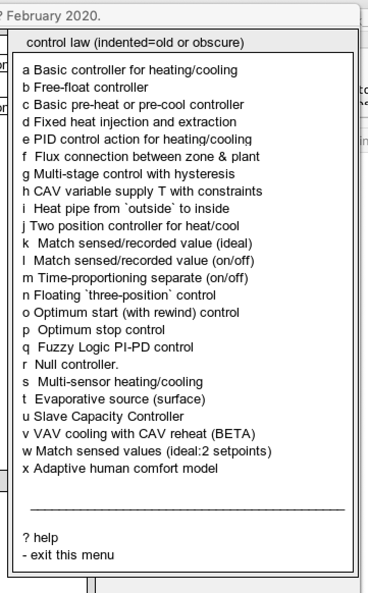
Simulation suites implement environmental controls via one or more arbitrary conventions:
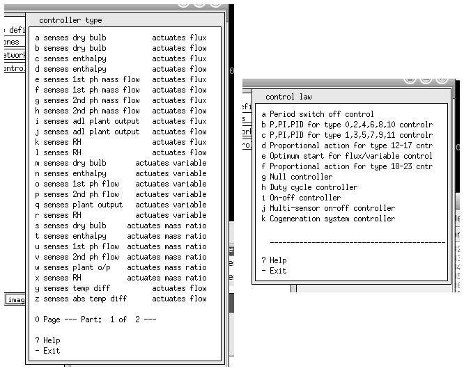
Idealised system representations:
Which define a generally recognised high level pattern (e.g. VAV terminals with a perimeter trench heater), via high‐level parameters which are then associated with a number of thermal zones in the model. The DOE‐2 simulation tool is a classic example of this approach. These often only roughly approximate what the practitioner has in mind. Practitioners are confronted by the black art of tweaking an existing system to mimic a different design variant.
Or of control logic which define what is sensed e.g. dry bulb air temperature, control logic that responds to the sensed condition and some form of actuation e.g. the injection of flux at some point in the model. Usually there are a limited number of parameters that can be set by the user and such controls tend to be applied to individual thermal zones. ESP-r supports this. These present users with a mix of abstract terms e.g. radiant/convective splits and behavior e.g. proportional/integral action rather than physical devices. Frustratingly, ideal zone controls often ignore the parasitic losses and electrical demands that many practitioners are interested in.
System components:
Libraries of components e.g. fan coils and valves, which can be assembled by the user into a variety of environmental systems as required and linked with control components and logic. There may be several representations with different levels of resolution - ESP-r seems to have a dozen variants of hot water storage tanks (accumulators). Some Tools use steady-state component representations whilst ESP-r uses dynamic components.
A component based approach allows more flexibility than pre‐defined systems but assumes that the practitioner can source the necessary attributes from manufacturers, has the skills to choose appropriate components and link them together correctly. ESP‐r supports networks of system components, optionally in conjunction with mass flow network components and electrical power networks.
Templates of components:
Some tools (but not ESP-r) use a template approach to expand a limited number of descriptive terms into scores, if not hundreds of components of a known topology, typically including control components and control logic. Templates often use a high level language to support the creation of component networks.
Practitioners are assumed to trust the topology and specifics of the resulting network. The QA and due dilligence implications are substantial. Adapting such a network for the needs of a specific project would require a deep understanding of its contents.
Here is a list of questions which might help identify whether a network of system components or an idealised approach is suitable at the current stage of the design process:
Do we have sufficient information to define an idealised or component approach?
Which approach can deliver our agreed performance indicators?
Can we explore broad‐brush and/or ’what‐if’ questions?
Can we tweak attributes during the detailed design phase?
Are we doing something outlandish like mimicking a radiant cooling system with ’purchased air’.
Does the documentation support QA tasks?
How human readable is the template-generated network?
What support is available to move from an abstract representation to one with a higher resolution?
Chapter 6 explores ESP-r’s facilities for idealized controls and Chapter 9 explores ESP-r’s facilities for component based environmental controls. There are several other simulation entities that also include control attributes. For example, mass flow network component control is discussed in Section 7.7
1.10 Design of assessments
A tactical approach limits the quantity of information we have to deal so both the model and its performance is easier to understand and the QA burden is reduced. Computers may process a year in seconds while staff discover opportunities and risk at a different pace.
One of the early planning tasks is to identify the nature of assessments which will allow us to gain confidence in the model and modelling approach as well as deliver performance indicators well‐matched to the design team goals.
Again we want to avoid the usual suspects when deploying numerical tools. For example, many tools default to annual assessments and thus entrap the practitioner in a data‐mining exercise.
A key initial objective is to support our own understanding of performance by looking at patterns in a limited set of data and so be able to spot glitches in our model as well as opportunities for improvements to the design (or the clients specification) as soon as possible.
A key tactic is to define performance metrics (e.g. what can we measure in our virtual world) early in the process. Some metrics e.g an energy balance within a zone, might contribute to our own understanding of the design and other metrics e.g. thermal comfort might be useful to report to others in the design team.
Delaying details
Many practitioners feel compelled to jump into the details of their usual environmental control system during initial assessments. A strategic use of simulation would first establish patterns of demand and then find a system that matches that pattern.
First observe how it works without mechanical intervention. Focus on demand‐side management ‐ exploring architectural options and alternative operational regimes. Focus on transition seasons and environmental controls that can cope efficiently with partloads and intermittent demands. Discover patterns that stress the building and explore how interventions that mitigate the extremes can be integrated into the design.
Strategies suggests the following methodology to build our understanding of demand-side improvements and give clues about potential environmental control strategies and kit: - Identify typical weather week in each season plus an extreme hot and cold week. - How often does the building work satisfactorily without mechanical intervention during each season-week? - Test demand-side improvements for each season-week. - Identify type(s) of environmental controls which address the observed patterns of discomfort and create a minimalist/idealised representations of each. - Check part-load performance during spring/autumn weeks for each control type. - Check extent of peak demands and then the frequency of discomfort during extreme weeks if each system is critically undersized. - Transition the best-working control to full detail and confirm performance during each season-week and extreme week prior to running annual assessments.
ESP‐r workshops typically devote as much time to exploring building performance issues as is spent on model creation. Simulation suites which do not include an interactive exploration facility will include a descriptive language to specify what performance metrics are to be captured during each assessment ‐ so learn that language!
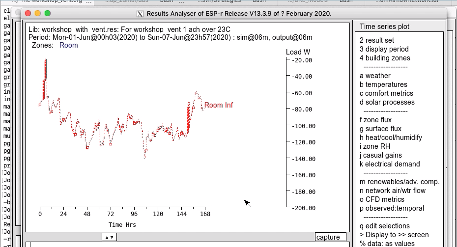
ESP‐r includes a results analysis tool res which scans the files which hold the domain‐specific predictions from an assessment e.g. building fabric results, electrical performance, mass flows and system components. This will be covered in detail in Chapter 10. Section 13.6 discusses the design of assessments which check if the building responds as expected.
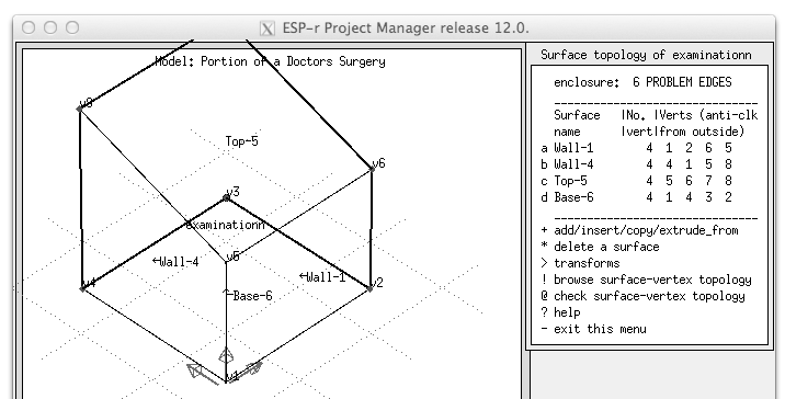
This review of planning tasks can now be tested in the context of a doctor’s office.
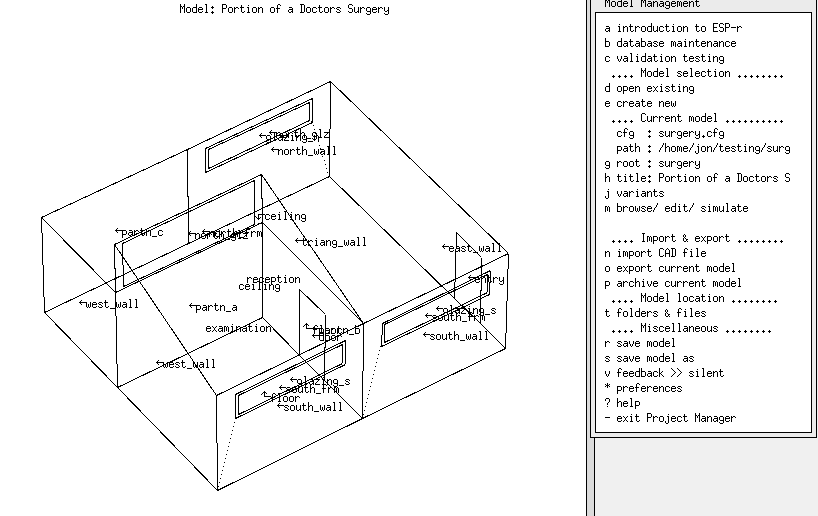
Chapter 2 BUILDING YOUR FIRST MODEL
For new users of simulation tools, the process of creating models will seem slow and will require seemingly endless requests for arbitrary information. An experienced user will, of course, do the same work in a fraction of the time. In ESP‐r workshops eight out of ten participants create models which simulate correctly the first time. Most are able to re‐create their initial model with minimal support and in ~25% less time. Let’s get to work!
This first simulation model involves refurbishment options for a general practitioner’s office (UK nomenclature, in other regions this is a neighbourhood medical centre). The client says the existing facility in Birmingham is sometimes uncomfortable and they would like to explore ideas for reducing heating costs. The client has limited resources and has requested rapid feedback on two initial ideas ‐ improving facade glazing and reducing infiltration. The client has a belief that this will result in a better working environment and the task for simulation is to test this.
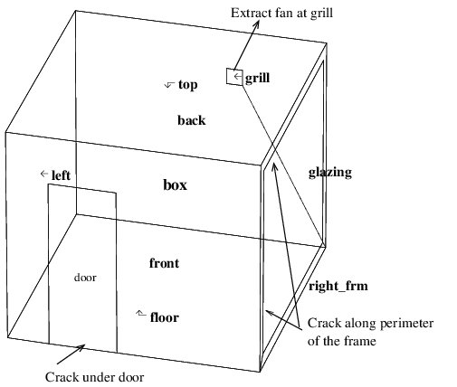
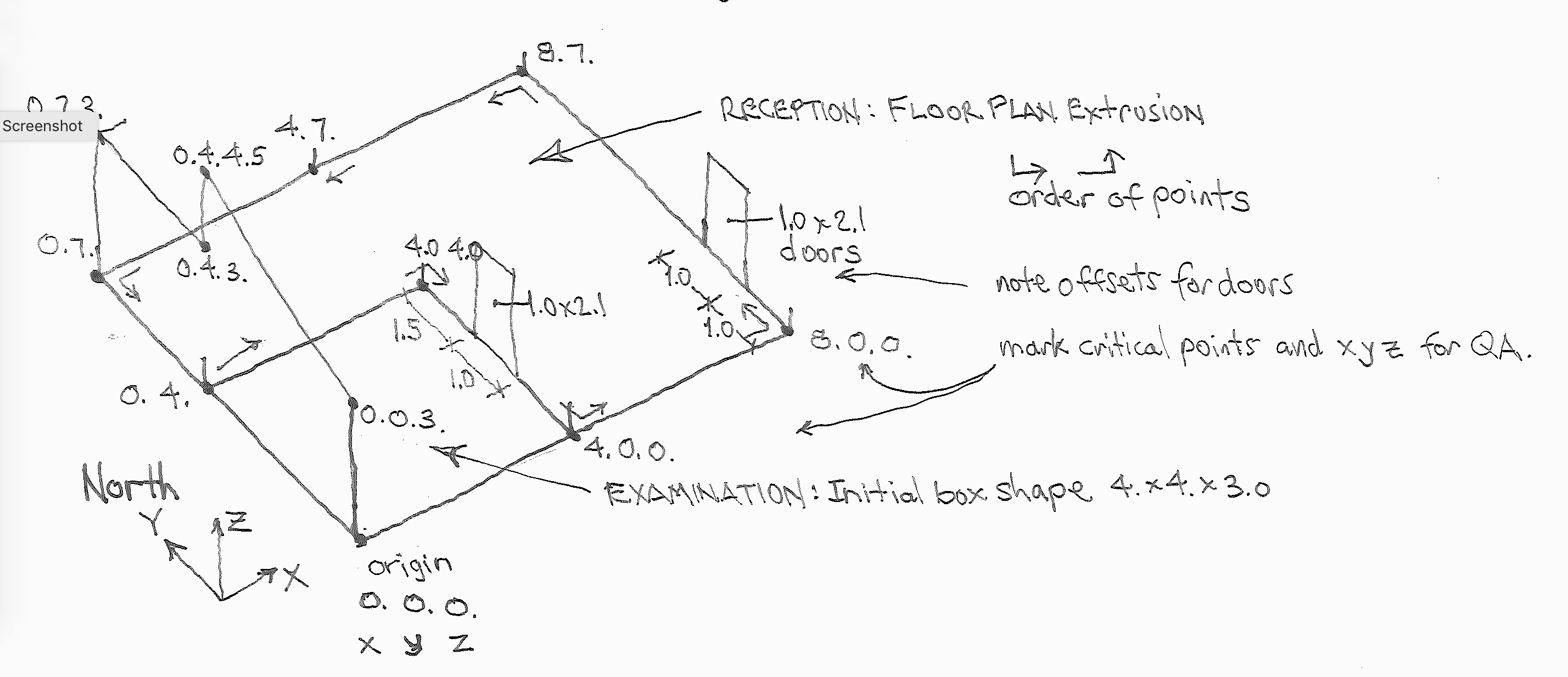
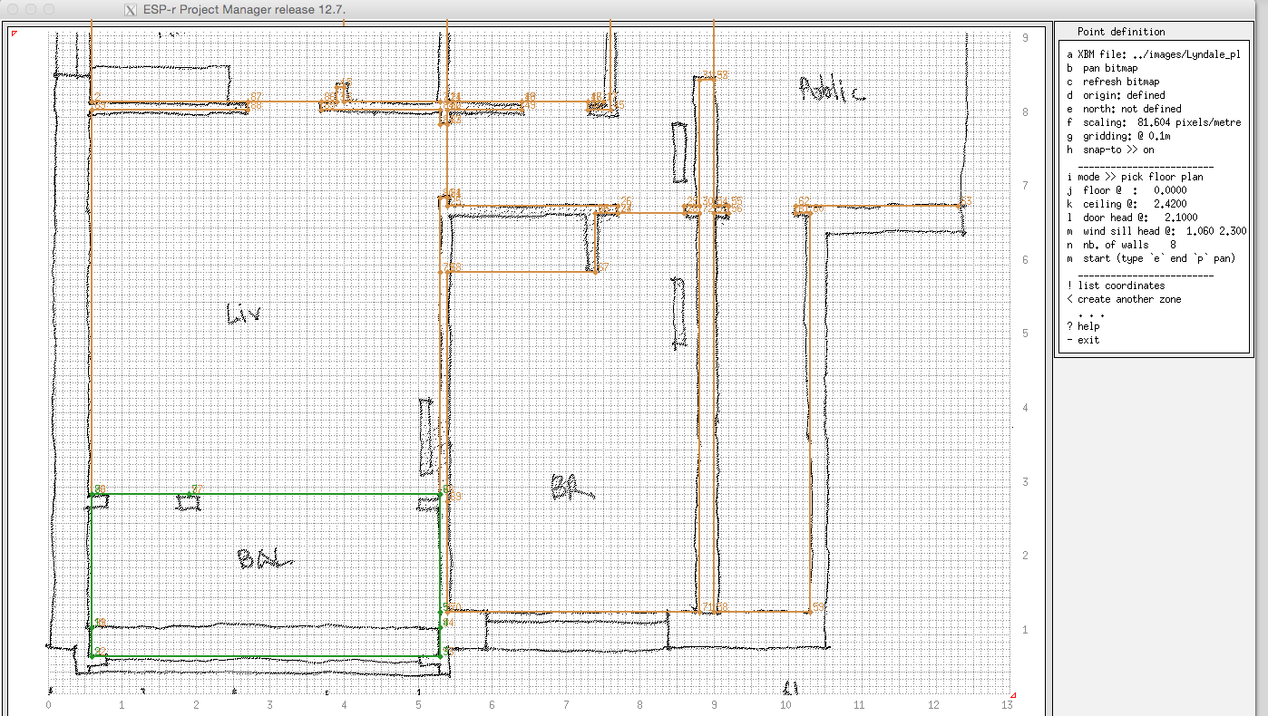
Figure 2.1 is a sketch indicating names, composition, critical coordinates as well as facade and door details. It also includes notes to support the creation and attribution of the model.
Figure 2.1: Overview of surgery.
The constructions are described as typical late‐1980s small scale commercial with masonry wall U values ~0.6, the flat roof of the reception U ~0.4 and the sloped roof of the examination U ~0.4. It has air filled non‐coated double glazed windows with U ~2.8 with wooden frames U ~1.6. The floor is slab‐on‐grade with carpet and no foundation insulation and a U ~0.7.
In Figure 2.1, the dashed lines at the upper‐left indicate another room which has similar environmental conditions but for which we have been given no other information. ESP‐r supports this level of abstraction via a boundary condition attribute ‐ in this case dynamic similar.
Initial information from the client is roughly two people in the examination room during the hours from 9h00 to 16h00 on weekdays with staff in until 18h00. The reception area serves other examination rooms and there might be up to five visitors plus a receptionist.
Further questioning elicits that Thursday afternoons are for staff only and the practice is also open Saturday mornings with up to seven visitors. Lighting in the reception is 150W during the hours of 8h00 to 19h00 and the examination room is 100W over the same hours.
Diversity is implied e.g. a lunch hour and a ramp‐up and ramp‐down of gains to represent cleaning staff in the morning and stragglers at the close of work. There should be periods with full loads so that capacity issues and the potential for overheating need to be addressed.
Our task is to translate this client description into the syntax of our simulation suite. ESP‐r represents casual gains as a schedule which applies to each defined calendar day type. By default there are weekdays, Saturdays, Sundays and holidays. For this model we need to add a Thursday afternoon staff-only day type.
Building facades have faults and the age and type of building suggests it is moderately leaky. There is a discussion about how the impact of infiltration and how it can be represented and assessed in the Flow chapter. For now let’s use an initial engineering assumption that there will be 0.5 air changes per hour (ac/h) infiltration at all hours.
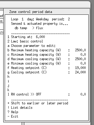
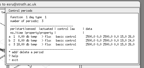
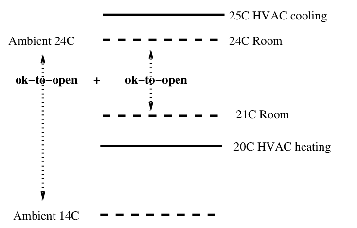
The heating set point is 21°C and the cooling set point is 23°C between 9h00 and 17h00 on weekdays with frost protection (15°C) at weekends and outside office hours. This is supplied via an air heating and cooling environmental control.
Let’s assume that we do not have a detailed specification of the components of the environmental control other than the set points, and that heating and cooling are delivered convectively. Since the design goal is to appraise changes in heating or cooling demand, not the control logic or system component performance, there is little point in providing detailed component descriptions.
Let’s use an ideal zone control to characterize the response of a convective heating and cooling system to the client’s set points. We do not know the capacity, so we will make an initial guess (say 4kW heating and 4kW cooling) and see how well that matches the demands.
2.1 Pre‐processing information
Get out your grid paper and note pad and keep the laptop lid closed for now.
Pre‐processing information and sketching the composition of our model will limit errors and make it easier for others to understand what we intend to create, and, after we have made the model, will help check that it is correct. This rule applies whether we are going to import CAD data or use the in‐built CAD functions of our simulation tool.
The XYZ coordinates in the lower left of Figure 2.1 take the centre‐line of partitions and the inside face of exterior walls, floors and ceiling and the origin of the model is at the lower left corner of the examination room. The critical vertical points to record on your notepad are 0.0 (ground), 2.0 (window sill), 3.0 (ceiling), 4.5 (top of sloped roof).
How much detail is needed? Look back at Table 1.1. The windows are not large and the questions are general. It is however necessary to represent the window frame accurately as it is one of the design variants the client is interested in.
Table 2.1 Method for general practitioner surgery
Design Question
Simulation Questions
What specifically do we want to know about the design?
Frequency and extent of discomfort as well as winter heating demand. Improvements from upgrading the facade glazing and reducing infiltration.
Does available information match tool requirements?
Check common data sources and review risks associated with our assumptions. Review available reporting options and discuss with client.
Model extent and level of detail?
Represent one examination room and the whole of he reception with adjacent spaces represented only as similar boundary conditions. Include facade frames and accurate glazing positions but do not bother with furniture, or doors to the un-represented adjacent spaces. Establish assessment periods used to confirm the impact of facade changes.
How will we know if a design idea is well-founded?
Is comfort improved? Are there noticable changes in heating capacity or demands? Are there changes during Monday morning startup on extreme winter mornings?
How might the design fail?
Overheating from internal gains is not mitigated by the upgrades. Lower infiltration might result in poor air quality or overheating.
What are the opportunities?
Alternative facade upgrades or overhangs.
Is our approach robust?
Double check model against initial sketches and planning documents. Consider who creates the model and who checks the work. Are occurrences of discomfort and environmental control demand as expected? Do these design changes impact other performance criteria? Have colleagues review the predictions.
2.2 Model registration
Time to take the client’s specification, planning sketches and notes and startup the simulation software (if you are using another simulation tool adapt as required).
Surgery is a clearer name than TEST1. And. Think. Before you press OK.
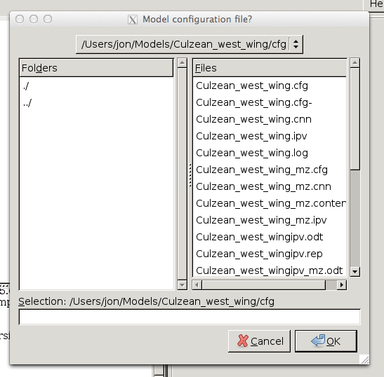
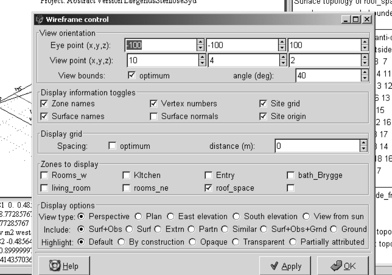
Exercise 2.1 will guide you through the model registration process. After you complete Exercise 2.1 the interface will look like Figure 2.2 and there will be a set of folders as in Figure 2.3.
Exercise 2.2 will guide you through a model archiving process. Archiving is a good habit. ESP‐r has few undo options so trigger points in work‐flow are needed.
Consider where your model is located and the nature of the site. Other than being in Birmingham and in an urban setting the context is poorly defined. Table 13.1 provides a checklist for site issues.
Document your site assumptions and links to site photographs or maps and store these within your model folder. Now is the best time to make the first archive of your model! And a good time to review the contents of the model folder to see where information has been placed.
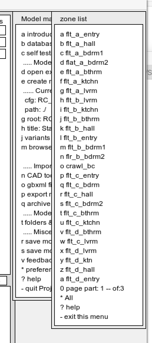
Figure 2.2: Model management and zones menus.
Figure 2.3: Naming pattern for ESP‐r model folders.
2.3 Review of weather patterns and common data
Having registered a new project there are several tasks to complete before defining the form and composition of the surgery:
Find a weather file and typical periods for our assessments.
Review common materials and constructions.
Select or create place holders for constructions and materials.
A tactical approach uses short weather sequences for model calibration and focused explorations. As examples, what can a Monday morning start‐up after a cold weekend tell us much about the characteristics of a building? If we reduce infiltration and improve the glazing will this increase the risk of overheating so lets identify some warm days to confirm this.
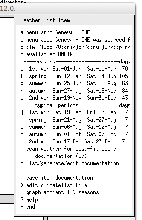
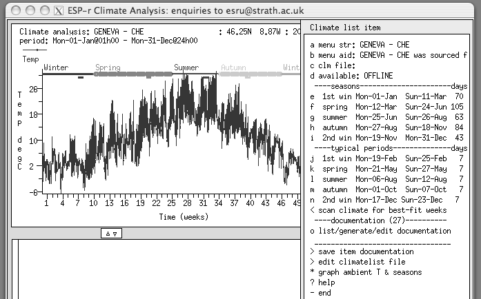
Most simulation suites include a weather analysis or review tool. The ESP‐r weather module clm provides facilities to explore weather data via graphs, statistics and pattern analysis facilities (see Section 3.1). Our initial task is to use these facilities to better understand the patterns in Birmingham and identify useful assessment periods.
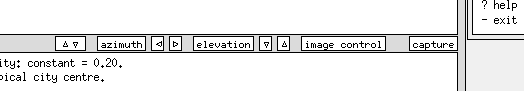
To work with clm, select the menu option Model Management ‐> Database Maintenance and in the options shown in Figure 2.4 select the annual weather option.
 Standard data maintenance:
   Folder paths:
   Standard <std> = /opt/esru/esp‐r/databases
   Model <mod> = no model defined yet
  _______________________________
a annual weather        : <std>clm67
b multi‐year weather    : None
c material properties   : <std>material.db4.a
d optical properties    : <std>optics.db2
e constructions         : <std>multicon.db5
f active components     : <std>mscomp.db1
g event profiles        : <std>profiles.db2.a
h pressure coefficients : <std>pressc.db1
i plant components      : <std>plantc.db1
j mould isopleths       : <std>mould.db1
k CFC layers            : <std>CFClayers.db2.a
l predefined objects    : <std>/predefined.db1
  _______________________________
? help
‐ exit this menu
Figure 2.4: List of ESP‐r common data stores.
Read Section 3.1 about search techniques for identifying an appropriate week in winter with a cold weekend, and a summer week with a sequence of warm days. For the surgery the Birmingham UK weather note the relevant periods to include in assessments.
2.4 Locating constructions for our model
Identification of constructions and materials prior to defining the geometry of the surgery forces us to consider aspects of its composition during planning and allow attribution of our model as we create it. While this should be a straightforward tasks do not be surprised if there are a number of complications: - Sections included in the construction documents may not be fit for simulation use, - Sections may provide insufficient coverage, - Specifications may include the dreaded or equivalent to achieve U=0.15
An early review can also identify relevant questions for the design team early in the process. In the surgery we have only a limited specification of the building composition. Our challenge is locate reasonable matches within the data stores.
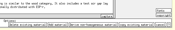
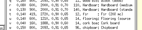
Chapter 3 provides an in‐depth discussion about common data files and the management of materials, constructions, optical property sets. It also how one might embed new information and record its provenance. In ESP-r, common materials are held in classes such as Brick, Concrete, Metal, etc. and each class holds a list of related materials as seen in Figure 2.5.
In projects we may need to adapt existing constructions by selecting alternative materials or creating material variants that match what will be used in a specific project.
Figure 2.5 List of materials classes and concretes.
For the surgery, read Section 3.4 (common materials) and Section 3.5 (common constructions).
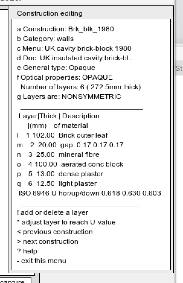
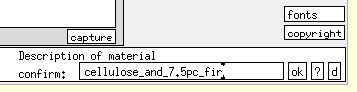
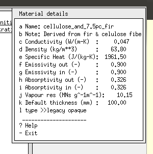
When you have done that, carry out Exercise 3.7 and Exercise 3.8 in order to locate the following entries in th standard common constructions file multicon.db) as shown below in Figure 2.6. In the video the construction search begins at 4m 50s.
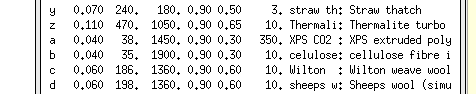
a floor which includes some ground layers ‐ grnd_floor carpet on sleepers over slab floor with earth below 0.975m thick U=0.699
a ceiling for the sloped roof of the examination room which also acts as a roof ‐ Pitch_rf1980 concrete tile pitched warm roof from mid‐80s 0.300m thick U=0.413
a flat ceiling/roof for the reception ‐ Flat_rf_1980 flat insulated light concrete with ceiling 0.204m thick U=0.390
2.5 Zone composition tactics
Most simulation suites provide at least a basic interface to define the form and fabric of the building and some have extensive in-built CAD facilities. In the Exercise we use ESP‐r’s in‐built CAD facilities. strategies recommends becoming familiar with tool facilities prior to the use of third-party CAD tools. Our tactical goal is to use a work-flow which minimizes the number of keystrokes and avoids errors:
plan for maximum re‐use of existing information
use the information in your planning sketches and notes
take opportunities to embed documentation in the model
give entities meaningful names and include attribution from the start
Of course you never lose scraps of paper and you always remember the assumptions you made four months ago and you will not be asked to demonstrate that you followed procedures.
QA works better if something that looks like a door, is named door and is composed of a door type of construction. Where attributes reinforce each other it is easy to notice if we get something wrong!
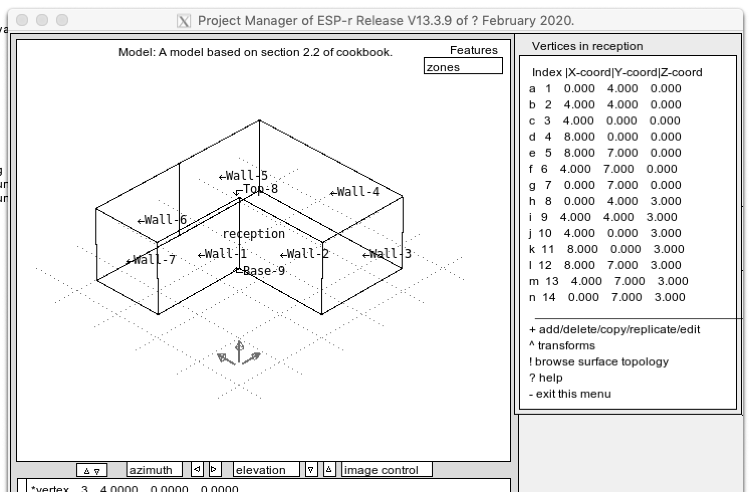
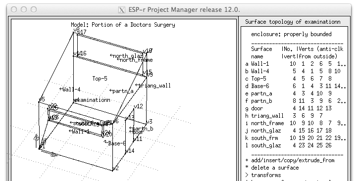
Simulation suites typically provide alternative methods for describing common room shapes. ESP‐r supports rectangular shapes (origin plus length/width/height and rotation), extruded floor plans (ordered list of points on the plan plus a Z value for the base and top) as well as general polygon enclosures. The eventual form of a room might be of arbitrary complexity involving hundreds of surfaces but the same underlying rules will apply.
The reception is L‐shaped and thus a floor plan extrusion is a good initial starting point. The examination room could be built from a floor plan or a rectangular shape into which we insert facade elements.
Figure 2.8 shows the development of the floor plan into the reception and subsequent transforms:
The initial floor plan of the reception is extruded into an enclosure with 7 walls, base and top.
The initial surfaces are given name attributes.
Doors are inserted into the partition and to the right facade of reception, named and attributed.
The rough‐openings for horizontal windows are inserted into the reception north and south facades using our chosen frame material.
The glazing is inserted (via frame facility) into the frames, named and attributed.
The surfaces in reception are attributed for composition.
The initial box for the examination is created.
The Z values for two vertices edited to form the sloped ceiling.
The right and back walls of the examination are removed.
The attributed partitions and door from the reception are copy‐inverted into the examination.
The triangular wall is created from the existing vertices, named and attributed.
The frame of the upper north window via existing vertices, then named and at‐ tributed.
The glazing for the upper north window is inserted at 80% of the parent, named and attributed.
The remaining surfaces of the examination are named and attributed.
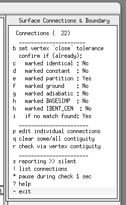
The topology check facility is run to define the boundary conditions for all surfaces.
This sequence supports the tactics outlined above, in particular the re‐used surfaces are already attributed and thus the attributes can be inherited. It takes less time to copy a partition and door than to re‐create and avoids the risk of misalignment. The exercises allow you to explore such sequences and after you gain experience you may find further tweaks to improve your work‐flow.
Surface considerations
Architectural elements should be included in a model if they are thermally important. Internal glazing, doors, structural elements and furniture may be of marginal interest. A tactical approach includes them if they make it easier for others to understand the model ‐ we save time because we do not have to explain why we have omitted entities.
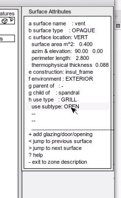
Surfaces are an entity type in all simulation suites. Each vendor has evolved their own arbitrary conventions so although surfaces are ubiquitious they are difficult to equate. ESP-r uses surfaces to represent just about everything: - A surface is a partition, ceiling, window, door, frame or grill if you give it a suitable name, attribute its composition accordingly and set its USE attributes. All surfaces fully participate in the analysis. - Surface polygons must be flat and have less than ~120 edges. - Window frames, architraves, skirting, cabinets and furniture are optional. You can explicitly wrap frames around glazing or architraves wrapping around doors or aggregate them into a few surfaces of equivalent area and composition. - Glazing or doors need not be child surfaces of another surface and can share edges with more than one surface. - A zone can be enclosed in another zone e.g. using a zone to represent a water filled radiator or water mass as long as the enclosing zone includes the shared surfaces of the inner zone(s). - Mass within a room can be represented by one or more pairs of opaque surfaces (back-to-back) of arbitrary polygonal complexity. - Linear thermal bridges can be associated with edges in the zone. - Solar radiation will pass through any surface facing the outside or another zone which has an optical attribute set to something other than OPAQUE or which references a Complex Fenistration Component.
An example rule set for EnergyPlus can be used as a comparison. Most simulation tools have a user contribution blog which provides hints.
Surface attribution
All simulation suites overload surface entities with attributes. All include a NAME attribute. Otherwise arbitrary conventions dominate and it takes considerable passion to establish equivalence between simulation suites. The ESP-r surface attribute convention is illustrated by Figure 2.7, which gathers most of the user defined and derived attributes. In a well-designed model surface attributes reinforce each other - i.e. if door_to_entr was composed of foundation_wall we would hopefully spot that something was amiss.
To name something is to own it.
In later sections we will discuss naming patterns that have been observed to work. Folk in a hurry often accept default names for entites. CAD tools are particularly opaque in their creation of names such as W-282-375-I-W-265. It might have only taken a few seconds to import an 80 zone model but then we have 1500 surfaces with similarly opaque names to work with.
Figure 2.7: Surface attribution.
The specific surface in the figure door_to_entr has the following user defined attributes: - Name (up to 12 characters) - Optical (name of an optical property, complex fenistration or OPAQUE) - Composition (name of a construction) - USE (a pair of KEY WORDS see below) - Environment (four indices representing the boundary condition) - Edge list (number of edges and a list of vertex indices)
The following attributes are derived from other information: - Location (VERT SLOP CEIL FLOOR) - Parent of & Child of (surface names or -) - Flow Component (name of associated flow component)
USE attributes are pairs of KEY WORDS to automate modifications to surface sizes or attributes e.g. a surface as a code compliant WINDOW. They also record the users intent e.g. STRUCTURE, PARTITION, FRAME (as pure documentation). Some KEY WORD pairs provide directives which inform the initial creation of mass flow networks and visual assessments. The combinations currently supported are:
DOOR CLOSED ‐ 2mm crack around perimeter, DOOR UNDERCUT ‐ orifice the width of the door of user defined height, DOOR OPEN orifice (full size) with discharge coefficient, DOOR BIDIR ‐ two way flow based pressure & temperature, DOOR ADJ-BIDIR two way flow for slightly ajar door. For the OPEN, BIDIR, ADJ-BIDIR a parallel crack connection is also created.
Fictitious surfaces low mass & transparent: FICT CLOSED or FICT CRACK - 1mm crack length perimeter of the surface, FICT OPEN ‐ orifice with use defined area, FICT BIDIR ‐ two way flow based pressure & temperature, AJAR FICT BIDIR two way flow with restricted width.
Frames associated with doors & windows: FRAME CLOSED or FRAME CRACK ‐ 1mm crack with length half of perimeter, FRAME VENT ‐ orifice 15mm * 400-700mm wide
small surfaces marking the position of grills: GRILL CLOSED or GRILL CRACK ‐ 1mm crack with length of perimeter, GRILL INLET ‐ fixed volume flow incoming, GRILL EXTRACT ‐ fixed volume flow extract, GRILL OPEN ‐ orifice with discharge factor, GRILL DUCT ‐ conduit with hydraulic diameter and local loss factors.
WINDOW CLOSED or WINDOW CRACK ‐ 1mm crack length is width of the surface, WINDOW OPEN ‐ orifice with use defined area, WINDOW SASH ‐ top and bottom orifices width of window, WINDOW BIDIR ‐ two way flow based pressure & temperature, WINDOW AJAR - two way flow with constrained width. For the OPEN, BIDIR, ADJ-BIDIR a parallel crack connection is also created.
FIXTURE + IESNA light distribution name is used in the creation of a Radiance lighting fixture
F-FRAME - (code compliant facade frame for use by 3rd party code compliance)
DOOR -P-DOOR - or V-DOOR (personel or vehicle door for code compliance)
D-WINDOW -S-WINDOW -C-WINDOW - (for use by 3rd party code compliance)
Using the planning sketch (Figure 2.1) and with reference to the geometric transforms (Figure 2.8) complete Section 2.3.
Figure 2.8 Sequence of geometric transforms for the surgery.
Figure 2.9 shows the reception after the initial extrusion of the floor plan. Notice that:
The zone geometry menu has been updated to reflect the new surface information. For example the volume of the reception is 120.0 m3 and the base of the reception changed to 40m2.
The text summary includes a synopsis of the geometry of the zone and a list of the attributes and derived values for each of the surfaces. You will notice that the word UNKNOWN shows up many times so there is still work to be done!
You will also notice that the surfaces have been given names like Wall‐1 and Base‐9. These are unambiguous without being particularly helpful.
Figure 2.9: And here is what it looks like after initial extrusion!
The viewing parameters for the wire‐frame geometry can be adjusted to alter the viewing direction, focus and the extent of information displayed. Control of the wire‐frame view is a basic skill which is covered in Section 2.4.
2.5.1 Doors and windows
Simulation tools offer a mix of options for representing doors and windows at different levels of resolution. Some simulation suites consider doors and windows to be child surfaces which inherit position and orientation from a parent surface. They may treat them as simplified thermophysical entities and frames as non-geometric attributes of the glazing. Tools may also embed support for alternative treatments of glass near framing or for advanced optical properties.
In ESP-r a window, door or frame is just another surface which fully participates in all heat flow paths. Parent-child relationships are derived geometric attributes.
Some practitioners will tend to abstract facade elements, for example lump all glass facing south in a room into a single surface as in the left of Figure 2.10 which was sourced from here. Facade engineers will often choose to be literal (upper right) including explicit representations of all frame extrusions in a 3D conduction assessments whilst others will choose moderate detail. If glare is of concern in the project then this would point to higher facade resolution.
Figure 2.10 Alternative facade approaches (upper right sourced from Achim Geissler at InterGGA).
How would you choose to represent the various facade details shown in Figure 1.2?
Establishing whether the mix of descriptive and analysis features supports a particular project is a non-trivial task. Check feature comparison sites or compose your own virtual tests to confirm what level of resolution is appropriate for specific simulation goals.
Issues to consider: - If a large pane of glass is used in a room with small surfaces then you may wish to subdivide the glass - Small dimensions may confuse view-factor calculations ‐ i.e. a frame 20mm wide around a 4m wide glazing. - If you are interested in local comfort or solar distribution then subdivide surfaces to increase spacial resolution and include furniture and fittings in addition to defining so-called MRT sensors. - If you are interested in glare then plan for a higher resolution facade.
Simulation tools often separate geometric and composition descriptions from directives associated with air flow. For example, ESP-r ONLY tracks air passing between rooms or with the outside if you intentionally create an air flow schedule or include relevant flow components within an air flow network. Some tools may create flow directives with minimal notification so check how your tool approaches this.
If your ESP‐r model is going to be exported to an application which has a different set of rules for windows include such criteria in the model planning. For example, Energy Plus requires glazing to be a child surface of an opaque parent surface. Test various approaches to find which works best.
Adding surfaces
Simulation tools usually provide a number of options for adding or inserting new surfaces - and they tend to manage the updating of related data structures and relationships. You will use these frequently so visit the exercise below and try out several of the variants so that you can plan your response to various building details. Some users like to hack the model files but this often introduces subtle errors and breaks the underlying dependencies within model files.
Exercise 2.5 inserts the entry door and the door to the examination room and then the frames and windows on the north and south facades.
Of course, at this point all of the initial entities have default names and many of their attributes are UNKNOWN. Surface attribution is the subject of the next section.
2.5.2 Completing attribution
To name something is to own it.
Tactically, we want to make it easy for others to understand our models. Clear names increases the speed and accuracy of selection from lists and clarifies reports. So attribute names of surfaces first.
One pattern that has been seen to work is roughly:
names like floor, ceiling, entry-door have almost instant recognition
if the floor or ceiling is represented by several surfaces then append a unique identifier e.g. floor-a, floor-b or floor-front, floor-bk
walls that face the outside might indicate which way they face via north-wall, east-wall but if a model might be rotated such names can be confusing so front-wall is better
naming partitions based on the zones on each side e.g. kitchen-partn, coridor-partn, some prefer partn-a, partn-b.
This pattern gives a clue about the location and composition of the surface. Note: non‐English names are ok as long as the ASCII character set is used.
Figure 2.11: Surface(s) attribution before and after.
Please review and explore Exercise 2.6 Attributing surfaces. ESP-r has a rich set of Surface Attribution which support both user documentation as well as driving a number of inferences as the model is created.
Figure 2.12: Reception after the addition of frames windows and doors.
2.5.3 Adding the examination room
The examination room is rectangular in plan, but has a sloped roof and it shares partitions with the reception. The geometric transforms in Figure 2.7 starts with a simple box shape, transforms it by editing coordinates to elevate the roof, deleting two surfaces and then copying surfaces from the reception and then using existing vertices to create the remaining surfaces.
The specific steps to add the examination room are the subject of Exercise 2.7. When you complete the exercise compare with your initial sketches. The transition from a box (in the upper part of Figure 2.8) to the room involves lots of steps and plenty of opportunities for error. The process of checking model details is covered in Sections 15.6‐15.9.
Figure 2.13: Examination initial box and surgery after attribution.
2.6 Model topology
Surfaces have attributes which define what happens at the other face in terms of a thermophysical boundary condition. In ESP‐r this attribute starts as UNKNOWN (see left Figure 2.14). One path for setting it is via Zone geometry ‐> surface attributes ‐> (list) ‐> environment ‐> surface boundary (list) The listed surface boundary options (see right Figure 2.14) are defined in the Entities Appendix.
Figure 2.14: Surface attributes and boundary options list.
And if there are many surfaces which have the same boundary condition e.g. they face the outside we could use the Zone geometry ‐> surface attributes ‐> attribute many ‐> boundary condition And there is also an automated process for this which we will explore shortly.
In the context of the surgery, the wall of the reception named partn_other in Figure 2.1 is facing another room for which there is no description other than that conditions are similar to that of the reception. For partn_other the boundary type would be similar to current.
The floors of both zones are slab‐on‐grade and are composed of grnd_floor (which includes 1m of earth) and it would make sense to use a monthly ground temperature profile. If we knew what the temperatures at 1m depth were we could enter these as a user defined ground temperature profile. Failing that we can select from one of the in‐built profiles.
In the exercises we initially defined a partn_a in the reception and made it out of the mass_part construction. We then performed a copy‐invert operation so that a surface with that name and composition exists in the examination. Clearly the two surfaces have a thermophysical relationship, however the copy‐ invert operation did not set the boundary condition, as can be seen in the right of Figure 2.14. This is intentional so that you remain in control of boundary conditions.
If you know which surface in another zone is the match then you can select surface in other zone but you might mis‐select which will cause all kinds of chaos. There is another option scan for nearby surfaces which will look for surfaces in other zones which are similar in size and have a likely orientation (~180 degrees from the current surface) and if there is only one match then it will set the boundary condition for this surface and the surface in the other zone as well. The scan for nearby surfaces is useful for the most simple models or in the case of a large model where changes have been made and you want to establish boundary conditions for a few selected surfaces. This does not scale well ‐ it requires lots of keystrokes as well as lots of mental attention. And, more importantly you might miss something. The better way is to use the ESP‐r topology facility.
The topology facility scans the polygons of a model looking for surfaces in various zones which are close matches in terms of shape and position and makes inferences from this to complete the boundary condition attribute of each surface. You control the tolerance and the extent of the search parameters and if the tool is unsure of what to do it will pause and ask for confirmation or allow you to select one of the standard boundary conditions.
To experience the automated process for establishing topology, take a few minutes to carry out the tasks in Exercise 2.8. Notice that every surface in your model is presented in sequence. It makes a great way to review your model. If you periodically invoke the topology facility (say after adding two zones) you will have a chance to review the model at the same time it is searching for matches to the new surfaces you have added.
Up to this point the strategy has been to follow procedures which help us to create correct models. How do we know they are correct? One of the steps in checking the quality of our models is to generate a QA report and then review this against our initial sketches.
Chapter 13 is all about model quality tasks. Now is a good time to read Section 13.9 which focuses on model contents reports as well as carrying out the steps for creating the report via Exercise 13.1 Exercise 13.1.
The report should be familiar to you ‐ it contains the entities that you cre‐ ated and named along with some derived data. If your review indicates that all surfaces are fully attributed then it is possible to proceed to the next step of instantiating the zone construction thermophysical properties.
2.7 Instantiating zone construction data
In order to run a simulation, each zone in a model must include full thermophysical data for each layer in each surface. Simulation tools embed this information in different ways. In ESP-r these are held in so‐called zone construction and zone tmc (transparent multi-layer constructions) files which are derived from the attributes of the surfaces and with reference to the common materials and common construction data associated with the model.
There is a one‐time task for each zone to initially build the zone files. Once these are in place subsequent changes to the zone or surface composition will trigger an automatic refresh. Follow the steps in Exercise 2.9 to create these zone files. If your initial zone geometry is properly attributed the task will only take a moment for each zone.
At this point we have defined the form and composition of the surgery using the basic facilities of ESP‐r. This is not the only approach we could have taken.
2.8 Geometry alternative inputs
Simulation tools may offer alternative schemes for creating the form and fabric of models. ESP‐r offers several options for geometric input:
in‐built CAD facilties for creating rectangular bodies, extruding floor plans or working with polygons
in‐built facilities (in the X11 interface version) to use mouse clicks on a regular geometric grid to define floor plans of rooms to extrud into zones with the option of including door jambs, window jambs and the origins of furniture and solar obstructions,
or to load monochrome images of plans and/or elevations, create a grid over them and click on points to define rooms, doors, windows, furniture origins or solar obstructions,
or importing gbXML files (a legacy DFX inport facility is being depreciated).
2.8.1 Clicking on a grid
In ESP‐r one option (via the X11 interface) is to define a regular X and Y grid and use this as the basis for establishing points for the floor plan of a building. Explore this via the re‐creating the surgery Exercise 2.10.
The planning stage for creating the surgery via a grid is essentially the same. The overall dimensions of the model are 8m (east‐west) and 7m (north‐south). Have Figure 2.1 available so you can complete the process in one session.
Exercise 2.10 focuses on clicking on points on a grid of the Surgery model. You will extrude both zones as well as their doors and windows in sequence and then use the normal geometric manipulation facilities to make the examination roof sloped and add the frames for the windows. This exercise helps you acquire the skills needed to use the click‐on‐grid facility (Figure 2.15).
After completing the exercise the two zones on the grid will be similar to Figure 2.16 (left) and in the wire‐frame view the steps remaining will be to create the frames for the glass and raise the ceiling of the examination room as well as adding in the clear‐story window.
Figure 2.16: After finishing the second zone.
2.8.2 Clicking on a bitmap
You can also supply your own bitmap of the building plan and click on points found in that image to create one or more thermal zones.
Practice is essential as is planning. The facility is intended to be used in a single session (points collected are lost when you exit the facility). So ALWAYS…
mark‐up your image with indications of the critical points you want to capture and the bounds of the zones you will be creating,
if you have bitmaps for more than one level in the building ensure critical points for the other levels can be identified or that the scale and origin of the other layer bitmaps are equivalent,
sketch your model in three dimensions so that you can plan how partitions between zones work.
For additional practice in clicking‐on‐plans (highly recommended) have a look at Exercise 2.11. There are any number of patterns that can be followed to achieve different levels of resolution. Keep a note of what worked for use in future projects.
2.8.3 Examples of approaches to take
Which ever simulation suite you are using, with practice you have the option to create create models which the client can recognize and which capture the spacial characteristics of the building. Two examples show the transition from sources to model:
The eighteenth century theatre shown in Figure 2.16 is an example of using scanned images of the building plans (there was no CAD data available). It is also notable in that almost nothing is rectilinear and many of the walls are ~1m thick.
The model in Figure 2.18 was initially composed by clicking on points from Figure 2.17 which were placed in dummy zones. Surfaces and points from those dummy zones were then used to build up the model zones. A detailed plan of the zoning and the critical points had been worked out first! Even with this, considerable care was required and post‐processing and reconciliation of the partition surfaces was needed. This is an example of what can be accomplished by an experienced user and is just the sort of project which would be cruel and unusual punishment for a novice.
Figure 2.17: Bitmap image from historic building.
Figure 2.18: Model of historic building.
The second example involves an urban study, as shown in Figures 2.19, which was largely composed by a digitizing on a mix of Ordnance survey maps, Google street view and spot site measurements. Some of the buildings are thermophysically complete and the others abstractions for context. Over time the high‐rise buildings will be populated. In this case the ground topology is treated as a thermal zone.
Figure 2.19: Layout and rendering of an urban setting.
2.8.4 gbXML inport
Importing third party model descriptive files involves establishing equivalence between the entities in such files and entities within simulation. DXF cad files include few attributes as well as many 2D entities that have limited application within simulation. gbXML file format is based on a richer data model from which a simulation model can be built.
ESP‐r facilities for parsing ASCII gbXML files are evolving. Sucess is dependent on the source of the gbXML file and the nature of design which is embedded within the file. Although the syntax of gbXML is well documented, vendors may implement sub‐sets of the standard. The mix of entities included may not fit within the ESP‐r data model i.e. surfaces with hundreds of edges are incompletely parsed. Sometimes the topology within the file does not conform to the internal rules of ESP‐r i.e. floors or ceilings edges do not join with edges of adjacent walls.
Exercise 2.12 explores the process of importing a gbXML file into ESP-r.
Figure 2.20: ESP‐r model after a sucessful import.
The new model might be incomplete. For example the parser will skip past surfaces or openings or doors which exceed array limits. And a gbXML file which contains non‐sensical forms will likely translate to an ESP‐r model with nonsensical forms.
Chapter 3 COMMON DATA STORES
Simulation tools tend to describe the composition of surfaces in terms of named constructions which are made up of an ordered list of materials (each of which have a set of thermophysical attributes). Each simulation suite has its own approach to implementing compositional information as well as providing user access for selection and management tasks. For example:
Energy Plus provides a folder with IDF files holding instances of window, frame, opaque wall and shading elements. The entries in these files are tag:data formatted. Users cut and paste relavent entries into the model file. Third party interfaces would provide these as selection lists.
IES VE provides lists of constructions by building type and, again, these reference named materials with thermophysical attributes.
ESP‐r is distributed with files which hold common materials, constructions, optical properties and other entities referenced within simulation models (see Figure 3.1). These files include ready to use entities as well as acting as templates for practitioners to populate from their own information sources. It is possible to configure ESP‐r to load an initial set of common data files that are appropriate for a given region and building type (see Install Appendix).
ESP‐r is also distributed with a collection of weather files which represent sites in many regions of the world. This collection can be extended via conversion of a number of standard weather file formats and user‐supplied definitions of seasons.
 Standard data maintenance:
   Folder paths:
   Standard <std> = /Users/jon/esru_jwh/esp‐r/databases
   Model <mod> = no model defined yet
   _______________________________
 a annual weather        : <std>clm67
 b multi‐year weather    : None
 c material properties   : <std>material.db4.a
 d optical properties    : <std>optics.db2
 e constructions         : <std>multicon.db5
 f active components     : <std>mscomp.db2
 g event profiles        : <std>profiles.db2.a
 h pressure coefficients : <std>pressc.db1
 i plant components      : <std>plantc.db1
 j mould isopleths       : <std>mould.db1
 k CFC layers            : <std>CFClayers.db1.a
 l predefined objects    : <std>/predefined.db1
   _______________________________
 ? help
 ‐ exit this menu
Figure 3.1 List of ESP‐r common data stores.
Note that each of the menu entries is proceeded with a <std> which indicates that the files are located in the standard ESP‐r distribution folder. Files in that folder should be treated as read‐only as many simulation models reference them. Variant files for a project should reside with the project and are preceded with a <mod> notation. Once selected a list of common management tasks (see Figure 3.2) is presented:
browse/edit ‐ work with the currently open file. Care is required when modifying files in the distribution database folder.
select file from list ‐ all of the files in the distribution database folder are presented and the one you select is associated with the model (not copied into the model folder). In the case of weather files the list is created from information held in a so‐called climatelist file.
select from model ../dbs ‐ any files in the model ../dbs folder are listed for selection
copy default file to model ‐ whatever file is specified as the default (via the defaults file) will be copied into the model folder and given an initial name consistent with the model root name.
create new ‐ writes a minimal contents file that can then be populated by the user as required.
Figure 3.2: Typical management options.
Details of weather, materials, constructions and optics common data files are discussed in the next sections.
3.1 Weather data
Organisations which gather, store and distribute weather data serve a broad audience. Over time a plethora of file formats have evolved. Simulation tools accommodated this via conversion utilities. The overhead for vendors and users was substantial as well as the risk of error and misunderstanding.
The author, with Dr. Dru Crawley, who at the time was managing the EnergyPlus program, designed and proposed the EPW weather file format which has become a widely used standard repository format for the simulation community with over 2000 locations available for download. EPW is a super‐set data model [ref] from which other tools can extract data.
Many of the weather files distributed with ESP‐r are sourced from EPW files. For sites which are not included in the distribution ESP‐r provides facilities to convert downloaded EPW files. Details of this and other import facilities are covered in Section 3.4
ESP‐r weather data is composed of a header which defines site information ‐ a name, year, latitude, longitude (degrees from the local time meridian) and a tag which defines whether solar data is measured as direct normal or global horizontal. Weather data is typically hourly for 365 days of the year but can be a fraction of the year. An annual ESP‐r simulation would begin in January and end in December. A whole‐winter assessment i.e. November to March would require a November‐December period and a January‐March period. Sub‐hourly weather data is accomodated via a temporal file (see Section 19.9).
At each hour the weather data comprises diffuse horizontal solar radiation, dry bulb temperature, direct normal or global horizontal solar radiation wind speed and wind direction with optional columns for atmospheric pressure. There are no entries for cloud type, cloud percentage, dew point, precipitation (or snow) or ground temperatures.
ESP‐r can also hold additional attributes of weather such as the start and end date for each season (winter beginning in January, spring, summer, autumn and winter ending in December) as well as a typical week for each season. Seasonal definitions are user specified and typical weeks can be determined via scanning of the weather data and this is the topic of the next section.
3.1.1 Exploring weather patterns
The use of short weather sequences for model calibration and focused explorations have many advantages. For example, a Monday morning start‐up after a cold weekend can tell us much about the characteristics of a building. Do peak summer demands coincide with the hottest day or is it a function of several hot days in sequence? There is little point in using an annual assessment to explore such issues and considerable advantage to identifying and using specific weather patterns for calibration and to support early identification of opportunities.
To work with weather, select the menu option Model Management ‐> Database Maintenance and in the options shown in Figure 3.1 select the annual weather option. This is followed by a selection of weather management functions including [select from list] (Figure 3.3). Assuming ESP‐r was installed correctly, you will now be presented with a list of known weather files.
Select an existing weather file such as Birmingham IWEC, look at the summary in the text feedback area and confirm the selection. The ESP‐r weather module (clm) will start, and your first task is to confirm the weather file name in the initial dialogue. After this the main menu of clm looks like the right section of Figure 3.3.
There are a number of options under synoptic analysis (Figure 3.4) which are useful for finding weather patterns with which to test a building. To generate a statistical report as in Figure 3.5, first select the weather data you wish to analyze e.g. dry bulb temperature and then the type of analysis e.g. maximum & minimum and then the reporting frequency e.g. day/week/month. Near the bottom of the is an option find typical weeks.
Figure 3.3: Weather options, available weather sets and Clm module opening menu.
This facility works as follows:
the average & total heating and cooling degree days (HDD & CDD) and solar radiation for each season,
for each week, average HDD & CDD and solar data is found and compared with the seasonal values and the week with the least deviation (using user supplied weighting factors) is reported. For this weather and with the default heating and cooling base temperatures the best‐fit weeks start on 27 Feb, 10 April, 19 June, 5 Oct and 4 Dec. Write these dates down and then go review these periods by graphing and/or gathering statistics about them.
The weather module has alternative views the data so see which ’view’ tells you the most!
The provision of different views of the weather data can assist in locating patterns and answering different questions that clients might pose. Time spent exploring this module can provide critical clues as to patterns that may be used in the design process.
An example is the graph of temperatures over the year (Figure 3.6) with the current seasons (as defined in the Manage climatelist menu on the right side of Figure 3.4) is indicated at the top of the graph. There are a number of times when it is below freezing, but the graph indicates that these tend to be brief. This might support the use of brief performance assessments for winter heating demands and capacity. It also indicates scope for testing whether a design might be optimized to cope with brief rather than extended cold periods.
Another example is Figure 3.7 where the psychometrics of the outside air have been plotted over the whole year for the same location.
Figure 3.6: Annual plot of temperatures.
Figure 3.7: Annual psychrometrics.
Identification of weather patterns supporting a Monday morning building warm‐up test is the subject of Exercise 3.1.
Identification of patterns supporting overheating assessments is also useful. E.g looking for the hottest day of the year. However, for some buildings it takes a sequence of warm days to stress the building. Indeed, for offices the gradual build‐up of heat reaches a peak on Friday even if it is not a particularly hot day. Exercise 3.2 allows you to explore this.
Many regions have two types of winter weather than stress buildings and their occupants. The first is clear and cold conditions. Solar radiation can offset colder temperatures and often the wind speeds are low. The second pattern is cloudy periods which tend to be milder for temperature but often have high winds. Identifying both of these patterns can have advantages over the usual coldest‐day‐of‐the‐year approach. Explore this via Exercise 3.3. Later when you come to define the assessments to be undertaken you can use this information.
3.2 Scaling assessments
ESP‐r has a number of facilities which allow us to scale our models and assessments ‐ so we get, for example, annual heating and cooling for a whole building without simulating every day of the year or every floor of an office building. These facilities evolved over time based on observations about how practitioners adapted their models and the assessments they commissioned to fit within their computational and staff resources.
For many building types there is a strong correlation between predictions over one or two typical weeks in each season and seasonal heating and cooling demands. This can be demonstrated by commissioning short period assessments and full season assessments and looking at the relationship between the two perfomance predictions. Commissioning full season assessments to determine scaling for a building does take time and so alternative methods were investigated. Over scores of projects it emerged that there were relationships that could be used to identify suitable short assessment periods. The key to this was in the practitioners definition of the extent of each season and search criteria for typical periods.
For many readers seasons are demarcated by four month intervals or by notes in a reference guide. If we pause to consider what constitutes winter in Hong Kong we might conclude that it is triggered by something other than temperature. The start of spring might be a day on a calendar but often there are cultural clues such as observing cherry blossoms which trigger changes in how we dress and how we operate our buildings. Astute practitioners leveraged this insight when they review weather data.
Before we had access to computers which supported numerical simulation simplified methods such as heating degree day (HDD and later cooling degree day CDD) methods were used. We observed that practitioners often did a quick check of HDD and CDD to judge, for example the onset of demand for environmental controls or the likely period that the building might be allowed to free float with minimal loss of comfort.
ESP‐r encapsulates this approach and extended it to also allow for solar radiation to be taken into account and weightings to be give to HDD, CDD and radia‐ tion. We will cover this topic later in the section about Integrated Performance Views (IPV).
 Degree day analysis: heating base at  17.0 cooling  21.0 Deg C

Winter (early year) season period: Mon‐01‐Jan@00h00 ‐ Wed‐28‐Feb@24h00
 Heat DD avg/day      14.91  Cool DD avg/day    0.00    Rad avg/day     1.23
 Heat DD avg/week    104.38  Cool DD avg/week   0.00    Rad avg/week    8.58
 Season heat DD      879.81  Season cool DD     0.00    Rad total      72.35

Spring season period: Thu‐01‐Mar@00h00 ‐ Mon‐30‐Apr@24h00
 Heat DD avg/day       9.08  Cool DD avg/day    0.00    Rad avg/day     3.47
 Heat DD avg/week     63.54  Cool DD avg/week   0.02    Rad avg/week   24.28
 Season heat DD      553.74  Season cool DD     0.18    Rad total     211.55
 . . .
Weightings for HDD CDD Solar: 1.0 1.0 1.0
Winter (early year) season.
period: Mon‐01‐Jan@00h00 ‐ Wed‐28‐Feb@24h00
 Week: 1 starting Mon‐01‐Jan DD total/week    108.02    0.00  Rad total/week    6.433
 Params (heat|cool|solar)    0.035    0.000    0.251 Params total     0.285
 Week: 2 starting Mon‐08‐Jan DD total/week    110.93    0.00  Rad total/week    6.087
 Params (heat|cool|solar)    0.063    0.000    0.291 Params total     0.354
 Week: 3 starting Mon‐15‐Jan DD total/week     98.08    0.00  Rad total/week    5.455
 Params (heat|cool|solar)    0.060    0.000    0.364 Params total     0.425
 Week: 4 starting Mon‐22‐Jan DD total/week    110.60    0.00  Rad total/week    6.781
 Params (heat|cool|solar)    0.060    0.000    0.210 Params total     0.269
 Week: 5 starting Mon‐29‐Jan DD total/week    100.02    0.00  Rad total/week    7.573
 Params (heat|cool|solar)    0.042    0.000    0.118 Params total     0.160
 Week: 6 starting Mon‐05‐Feb DD total/week     91.16    0.00  Rad total/week   14.203
 Params (heat|cool|solar)    0.127    0.000    0.655 Params total     0.781
 Week: 7 starting Mon‐12‐Feb DD total/week     97.52    0.00  Rad total/week    8.661
 Params (heat|cool|solar)    0.066    0.000    0.009 Params total     0.075
 Week: 8 starting Mon‐19‐Feb DD total/week    110.82    0.00  Rad total/week   11.682
 Params (heat|cool|solar)    0.062    0.000    0.361 Params total     0.423
 Week: 9 starting Mon‐26‐Feb DD total/week     52.66    0.00  Rad total/week    5.471
 Params (heat|cool|solar)    0.496    0.000    0.363 Params total     0.858

 Best week number is   7 Mon‐12‐Feb with HDD of  97.52 CDD of   0.00

early winter ratio of season/assessment days:  8.000
early winter ratio of season/assessment heat DD:  9.022 cool DD: 1.000
Use best‐fit week for the 1st winter season?
Figure 3.9 Winter fit criteria.
The method embedded in the ESP‐r weather module clm codifies the manual techniques and is illustrated in the listing Figure 3.9. Weather data is scanned week by week for the average HDD and CDD for each day and the total for each week as well as the daily mean direct and diffuse solar radiation. To allow fine‐tuning of the scan the user can provide weighting factors for HDD, CDD and solar radiation as well as the base temperature for HDD and CDD. The weekly data are then compared with the average and total values for the season and the week with the least deviation is suggested as the best fit.
Model calibration exercises that use such best‐fit weather patterns in each season can provide a reality check which is both constrained in computational time but sufficiently focused for staff to notice patterns that would not be evident in a worst day winter/summer assessment.
To make it easier for practitioners to use selected weather patterns ESP‐r support META data about seasons (early‐year winter, spring, summer, autumn, late‐ year winter in the Northern Hemisphere, early‐year summer, autumn, winter, spring later‐year summer in the Southern Hemisphere) as well as typical assessment periods.
3.3 Defining seasons and typical periods
When working with a weather file which is already selectable in the Project Manager weather list it will already have meta data defining the duration of each season as well as a typical week in each season which can be used for short duration assessments.
The concept of a season can be leveraged in several ways. The clm module provides a number of views of weather data, including statistics, which can help you identify weather patterns which conform to your own definition of seasons.
Exercise 3.4 in the Exercise Appendix explores different reporting options to identify that start and end dates for seasons of the year that are consistent with local preferences. You can also scan weather data for find the best fit week for each season using a combination of temperatures and solar radiation.
When you have completed the exercise you will a seasonal display such as Figure 3.6 which shows the seasons along the top and the ambient temperatures on the graph below.
Once you have explored seasons you can record the information in a block of text that can be included in the so‐called climatelist file. Exercise 3.5 goes through the steps of creating this block of text and it also provides information about the format of the climatelist file.
3.4 Importing weather data
Although ESP‐r is distributed with several dozen weather files (in the climate folder of the ESP‐r distribution) associating new weather data so that you can select it quickly and use it robustly within projects requires a number of steps.
The instructions in Exercise 3.6 in the Exercise Appendex allow you to install a new weather file, specify the days in each season and then use clm facilities to discover typical assessment periods in each season.
A good source of weather data is the United States DoE web site which is located at the following site. The site offers US locations, Canadian Locations and International Locations.
3.5 Common materials
Common materials files hold information on material thermophysical properties. These are held either in the ESP‐r distribution database folder or in a model’s dbs folder in the case of project specific materials.
As seen in Figure 2.5, materials are held in classes e.g. Brick, Concrete, Metal. A category such as Concrete, contains general types of concrete such as heavy mix concrete and adapted materials such as which painted heavy mix which has adjusted surface properties to represent painted surfaces.
Each material has the following attributes:
name is a short identifier
description ‐ block of text describing the material, the material name and the initial portion of the material descrition are included in the construction definition
conductivity (W/(m‐K))
density (kg/m^3)
specific heat (J/kg‐K)
emissivity in the long wave band (‐)
absorptivity in the short wave band (‐)
typical thickness (mm)
tag indicating whether it is opaque, transparent, or a gas.
ESP‐r differs from other tools such as DOE‐2 and EnergyPlus in that materials are only given a specific thickness when they are associated with a construction layer. Thus a single brick material might be used in several constructions with different thicknesses.
Exercise 3.7 is about navigating the categories of materials and searching for items. When adding new materials it is recommeneded that you document the source of the thermophysical data as well as any assumptions made within the material description. Any changes you make will be held in memory so the ! SAVE materials database entry should be used frequently. If you need to evolve a materials database for purposes of a specific project then make a local copy of the materials file via the copy default file to model or copy file from common to model options.
The category named GAPS is included to signal a non‐solid layer which is treated as a resistance to heat flow (for vertical and sloped & horizontal positions). For example, a low‐e coating in glazing increases the resistance to heat flow across the cavity and the resistance values would reflect this. Unless you are working with non‐homogeneous constructions where an air gap is represented as a conductivity, stick with the first air gap material (see figure 3.11) and supply the resistance values for the standard orientations.
Figure 3.11 List of GAP materials.
Normally, a simulation group would seek to protect their common materials from corruption. One way to do this is to insist that new materials or material variants are held in model‐specific materials files and only incorporated in the distribution common (database) folder by trained staff.
In the next section Figure 3.12 (and the listing on the next page) shows a raised floor system over a thick concrete slab. If we needed to include this in a model we would review the specification of the materials, see if there was an equivalent material. Let’s say that the raised floor is a Kingspan RG Series Gravity Lay access floor <www.kingspanaccessfloors.co.uk/>. The product is made up of 2mm steel, 28mm of high density particle board and 2mm steel. Generally carpet of 8mm is laid on top.
The materials database only has medium density boarding so we must search for data on high density particle board. There is an entry in Thomas Irvine’s Handbook of Heat Transfer which list a density of 1000 kg/m^3 and specific heat of 1300 J/kg.K and conductivity of 0.17 W/m.K.
To limit risk we want to create the new material in a common materials file associated with our model. Later we can get this incorporated into a corporate database. The steps required to copy a standard materials file into a model is covered in Exercise 3.9.
*item,HighDensityParticleBd, 91, 4,HDF based on info in Handbook of Heat Transfer by Thomas Irvine
0.170,1000.000,1300.000,0.900,0.900,0.700,0.700,55.000,9.0,‐
# layers  description  type  optics name   symmetry tag
    4     flr_ov_pln    OPAQ  OPAQUE       top_pln
# material ref thickness (m) description & air gap R
   42     0.0020  steel : Steel
   91     0.0280  HighDensityParticleBd : HDF based on info in Handbook of Heat Transfer
   42     0.0020  steel : Steel
  228     0.0050  grey loop pile : Grey loop pile synthetic carpet
Non-homogeneous materials
The above examples relate to homogeneous layers used in constructions. Often we need to represent layers which are a mix i.e. wood studs within a partition or floor construction but do not have the resources to implement 2D or 3D conduction. We have the option to define a new material which is a mix of two other solid materials, or by converting an air gap to an equivalent conductivity we can also represent walls which include voids.
Exercise 3.11 creates a new material which represents a cavity in a gypsum board partition which has 7.5% wood studs.
3.6 Common Constructions
A common constructions file holds categories of constructions such as opaque walls, partitions, frames, doors, fittings, earth etc. Vendors often include region-specific construction files so it is useful to spend time exploring their contents.
In ESP-r, several hundred constructions can be accommodated and thus the interface includes a number of management facilities. Files are located in the databases folder of ESP-r but may also be placed in the model dbs folder. It includes support categories as well as longer names and documentation for each construction (also referenced as a MLC).
A construction has the following attributes:
name ‐ up to 32 characters, must be unique, used internally and in reports
menu entry ‐ up to 32 characters to clarify selections from a potentially long list
documentation ‐ up to 248 characters describing the source and provenance of the construction.
category name ‐ the name of the category it relates to
optical property name or the key word OPAQUE
number of layers ‐ up to a dozen
for each layer the name of the material and its thickness
if layer is air then resistance to heat flow for horizontal, vertical, and sloped positions
tag indicating whether construction is symmetric
name of associated reversed layer construction
You may notice that reports about constructions include U values for the case of horizontal flow, vertical and sloped heat flow. These are derived values following conventions of ISO 6946. U‐values are not used within assessments (they are a steady‐state concept) but are included for purposes of comparison. Similarly glazing is often described with a G value which is a common reporting convention.
If you are reading this section in preparation for creating the surgery in Section 2.2 the planning phase requires the identification of constructions which match a description e.g. a window frame or door and a desired U‐value. Exercise 3.8 guides you through the process. Review the reports as entities are selected to confirm the overall thickness of the construction, the placement of mass and insulation. Constructions which have an optical attribute will include optical properties.
Physically thick layers e.g. stone in castles and the ground under a foundation need to be subdivided. For example, in the list in Figure 2.17 the grnd_floor has multiple layers of Common Earth which add up to 1m. Splitting a material in to several layers is a common technique for massive materials or insulation materials. It results in more nodes so the numerical solution is more efficient as well as providing higher resolution reporting of conditions within constructions.
Details of opaque construction: Brk_blk_1980 and overall thickness 0.273
In category walls also shown in menus as: UK cavity brick‐block 1980
UK insulated cavity brick‐block wall circa 1980 hard plastered.
Layer|Thick|Conduc‐|Densi‐|Spec|IR  |Solar|Diffu| R    | Kg |Description
     |(mm) |tivity |ty    |heat|emis|abs  |resis|m^2K/W| m^2|
Ext   102.0    0.77  1700. 1000. 0.90 0.70   12.  0.13 173.4 Brick outer leaf : Brick...
   2   20.0    0.00     0.    0. 0.99 0.99    1.  0.17   0.0 air  0.17 0.17 0.17
   3   25.0    0.04   105. 1800. 0.90 0.60    1.  0.62   2.6 mineral fibre : Mineral fib...
   4  100.0    0.24   750. 1000. 0.90 0.65   10.  0.42  75.0 aerated conc block : Aerate...
   5   13.0    0.50  1300. 1000. 0.91 0.50   11.  0.03  16.9 dense plaster : Dense plast...
Int    12.5    0.16   600. 1000. 0.91 0.50    8.  0.08   7.5 light plaster : Light weigh...
ISO 6946 U values (horiz/upward/downward heat flow)= 0.618 0.630 0.603 (partition) 0.585
Weight per m^2 of this construction 275.45

Details of transparent construction: dbl_glz with DCF7671_06nb optics & overall thickness 0.024
Layer|Thick|Conduc‐|Densi‐|Specif|IR  |Solar|Diffu| R    | Kg |Description
     |(mm) |tivity |ty    |heat  |emis|abs  |resis|m^2K/W| m^2|
Ext    6.0    0.76   2710.  837.  0.83 0.05  19200.  0.01 16.3 plate glass : Plate glass...
  2   12.0    0.00      0.    0.  0.99 0.99      1.  0.10  0.0 air  0.17 0.17 0.17
Int    6.0    0.76   2710.  837.  0.83 0.05  19200.  0.01 16.3 plate glass : Plate glass...
ISO 6946 U values (horiz/upward/downward heat flow)= 2.811 3.069 2.527 (partition) 2.243
Weight per m^2 of this construction  32.53

 Clear float 76/71,    6mm, no blind: with id of: DCF7671_06nb
 with 3 layers [including air gaps] and visible trn: 0.76
 Direct transmission @ 0, 40, 55, 70, 80 deg
   0.611 0.583 0.534 0.384 0.170
 Layer| absorption @ 0, 40, 55, 70, 80 deg
    1  0.157 0.172 0.185 0.201 0.202
    2  0.001 0.002 0.003 0.004 0.005
    3  0.117 0.124 0.127 0.112 0.077
 Total area of dbl_glz is      9.83

Details of opaque construction: grnd_floor and overall thickness  0.975
In category ground also shown in menus as: carpet conc floor hardcore‐earth
An uninsulated slab on grade foundation over hardcore and 600mm of earth with a built‐up of
chipboard and carpet above.
 Layer|Thick |Conduc‐|Density|Specif|IR  |Solar|Diffu| R    |Description
      |(mm)  |tivity |       |heat  |emis|abs  |resis|m^2K/W
 Ext   200.0     1.280   1460.   879. 0.90 0.85     5.  0.16 Common_earth
    2  200.0     1.280   1460.   879. 0.90 0.85     5.  0.16 Common_earth
    3  200.0     1.280   1460.   879. 0.90 0.85     5.  0.16 Common_earth
    4  150.0     0.520   2050.   184. 0.90 0.85     2.  0.29 Gravel based (non‐hygro)
    5  150.0     1.400   2100.   653. 0.90 0.65    19.  0.11 Heavy mix concrete
    6   50.0     0.000      0.     0. 0.99 0.99     1.  0.17 air    0.17 0.17 0.17
    7   19.0     0.150    800.  2093. 0.91 0.65    96.  0.13 Chipboard
 Int     6.0     0.060    186.  1360. 0.90 0.60    10.  0.10 Wilton weave wool carpet
 ISO 6946 U values (horiz/upward/downward heat flow)=  0.699  0.714  0.680 (partition)    0.657
Figure 3.8 Examples of common constructions to be used in the surgery.
Constructions are defined from the outside (the other face) working inwards towards the room face. If a construction presents the same order of layers looking from the room side or from the other side then it is SYMMETRIC.
Figure 3.12 Section of raised floor system.
An example of a non‐symmetric construction is the intermediate raised floor shown in Figure 3.13. Looking from the room below the ’other’ face is carpet and the room face is white painted concrete. From the room above the ’other’ facde is the white painted concrete and the room face is carpet.
The raised floor system includes a significant air space/layer. If the air space acts as a supply or return plenum then it might need to be represented explicitly as a thermal zone. In this case there are additional constructions listed below would be required:
Looking down from occupied space ‐ 32mm raised floor (other face), 5mm carpet (inside face).
Looking up from the plenum ‐ 5mm carpet (outher face), 32mm raised floor (inside face)
Concrete slab is the same from both viewing directions.
It is important to name constructions in a way which will allow reliable selections. In the above cases if we consider the observers position and look at the construction the names below might work:
floor_raised or room_to_raised ‐ looking down from occupied space to lower occupied space
ceil_raised or ceil_to_raised ‐ looking up from lower occupied space to upper occupied space
floor_over_plen ‐ looking down from occupied space to floor plenum
ceil_under_plen or slab_275 ‐ looking up from lower occupie space to floor plenum
top_pln ‐ looking up from plenum to upper occupied space
3.7 Common optics
Constructions which are transparent require additional attributes to describe how solar radiation passes through (or is absorbed in) the layers of a construction. Information to support this is held in common optics files either in the databases folder of the ESP‐r distribution or in a model’s dbs folder.
Common optics files hold a list of optical property sets. Each optical set has the following attributes:
name (up to 12 characters with no space), typically single layer optics start with an S, double glazing starts with a D but you can use any naming convention.
description (block of text up to 36 characters)
visible transmittance for use in exporting models to Radiance and for day‐ lighting calculations
solar absorption and reflection at the outside face for documentation pur‐ poses
U values for documentation purposes ‐ manufacturers data is often input here so the user can compare with the calculated U value found in the common constructions
number of layers (air gaps are considered separate layers)
five angular data for direct solar transmission (normal to the surface and at 40°, 55°, 70° and 80°)
five angular data on heat gain factors for documentation purposes
For each layer the angular solar absorption factors are held (at the same five angles as direct solar transmission).
Populating common optics files requires the use of third party software such as LBL Window 7. These produce reports which document the overall optical properties as well as layer‐by‐layer optical properties. These reports can be imported into an ESP‐r common optical file. It is up to the user to create a matching construction. Care is requied to ensure that any air gaps in the construction have appropriate resistances defined so that the reported U value matches the documentation in the optical data set.
ESP‐r supports control of optical properties within the zone construction facility (look for transparent layer properties ). This allows you to asso‐ ciate an alternative optical property set that is used if certain logical con‐ ditions are met. A simple example is a double glazing unit with a mid‐pane blind. One optical set might represent the blind in an open state and another with the blind partly closed. Both optical states should have the same number of layers.
3.8 Complex Fenistration Components
An alternative to the standard ESP‐r optics database, which holds moderate levels of optical attributes and resolution, is the concept of Complex Fenistration Components. The work which was originally carried out in Canada, attempts to represent a variety of facade build‐ups which include blinds as well as offering a more explicit treatment of heat transfer within gaps in glazing. In many cases the entities in the CFD database support black‐box treatments which solve the optical and thermophysical transfer within glazing systems and pass information back to the solver. A classic case is a blind which is mounted in the room with an air gap between itself and the glass. Without explicitly representing the gap as a zone it is difficult to represent the heat transfer at the blind. CFC2 in the attributes of the surface.
The figures above and below show views of the CFC database, categories of entities, entity lists and the attributes of a typical entry. There are hundreds of different manufacturers data sets which have been extracted from the IGDB. Constructions when they are built up point to these layer entries and the solver uses their attributes. When a room surface uses a CFC related construction the CFC solver is used rather than the standard optical code and the surface attribute shows up as a
Figure 3.13 Complex Fenistration Components selection and use.
3.9 Common pre‐defined entities
ESP‐r treats explicit thermal mass with the same level of thermophysical detail as facade surfaces. And while there are facilities to create internal mass pairs ‐ doing this from scratch is tedious, prone to error and does not scale well. Visual assessment tasks would be enhanced if one could populate the Radiance model with visual entities during the export‐to‐Radiance step rather than having to hack the Radiance files. And there are building entities such as stairs which are tedious to create but which, if absent, may mis‐represent the inertia within the building.
ESP‐r thus includes a database of pre‐defined entities which have the following attributes:
short name, text entry for list selection
blocks of descriptive text includes notes on use, applicability and provenance
intended domains e.g. visual, mass, zone‐enclosure
origin and bounding box (for preview)
list of vertices
list of mass pair surfaces (name, composition, optical properties, bounding edges)
list of boundary surfaces (name, composition, optical properties, bounding edges)
list of visual entities (origin, length/width/height, rotation, name, composition
list of named objects with associated visual entities
Pre‐defined entities are accessed via the databases menu as shown below:
Below are two typical entities. The first is an office chair which is made from 8 vertices, two pairs of thermal mass and 13 visual objects. These are intended to be imported into a thermal zone as required to populate the space for purposes of both thermal and visual assessments. An office space might have a dozen such entities, each will be given a unique name and thereafter will fully participate in insolation and long‐wave radiant transfers.
The second is a residential stair which, when imported into a model forms a complete thermal zone (there is a matching entity for the space above the treads). Other zone‐based entities include an explicit room thermostat (including an explicit thermistor, circuit board and case).
Figure 3.15 Pre‐defined office chair and stair zone.
Entities are typically created within ESP‐r as zones with whatever mass and boundary and visual entities required then transformed to the origin. The zone file can then be imported and documentation added to the entry.
Chapter 4 THERMOPHYSICAL RESOLUTION
This chapter is written from the author’s perspective as a Passive House trainer ‐ a standard with an extreme focus on building sections, especially the joins between facade elements. As an Architect and consultant the author has also noted the complexity of the built environment:
complex junctions which are not well represented by 1D heat conduction
exceptions to standard sections i.e. where structural elements are found at non‐standard spacing
instances where the external surface area of a facade differs from the inside surface area e.g. deep facade frame extrusions, window reveals and frames
thermal bridges which degrade the performance of building sections
instances where facades are geometrically thick rather than thin planer forms.
Unfortunately, some building sections form explicit instructions for future failure (e.g. condensation, micotoxin growth, local discomfort). With good pattern matching skills Architects can identify and correct inappropriate building sections prior to construction and contractors can identify and avoid faults. Simulation models often reflect little of this complexity and are thus unlikely to provide numerical clues as to future failures.
The geometric forms discussed thus far use polygons as the building blocks of our virtual built environment. While modern (thin) constructions, such as those used in Figure 1.5 are often approximated by conventional polygons, historical buildings (see Figure 1.6) and the thick walls and insolation seen in Figure 4.1 highlight the limitations of this convention.
Focusing on Figure 4.1, there are several aspects of the section which need to be considered during the planning and creation of models:
the thickness of insulation is substantial and in some places tapering
the wall section comprises a number of material types
the overhang (and window reveals) act to shade the facade of the building
the overhang forms a boundary for the upper section of the wall.
there appears to be an air space below the tiles which is separate from the air within the roof space.
above the tapering insulation is a channel for eaves air to mix with the roof space
it is not clear from the section whether the roof ridge is ventilated.
the area at the top of the insulation layer is somewhat different from the surface area at the ceiling.
Figure 4.1 Section and view of a low energy house
The list of bullet points could be much longer. We need strategies for ranking thermophysical issues and deciding what needs to be included in our model(s).
4.1 Modelling approaches
A tactical approach to simulation uses the planning phase to constrain options. The following is one possible ranking of what to preserve while abstracting a design into a model:
the volume of air
the slope of the roof
the location of mass within constructions as well as occupied spaces
the surface area in contact with the air
By default, most whole‐building simulation tools default to one‐dimensional conduction. The thickness of the insulation in Figure 4.1 thus poses a challenge. Do we choose to ignore the ceiling thickness when defining geometry? Use of physical co‐ordinates would help to preserve the volume of the roof space and the surface areas although this takes more time.
A high resolution model might sub‐divide the roof space to have an upper and lower section so that the temperature near the peak of the roof can be different from the air adjacent to the insulation layer. It might also include linear thermal bridge descriptions if these had been calculated.
A medium resolution model might subdivide the surfaces to represent full thickness and the partial thickness insulation and extend the roof zone to allow it to form a boundary at the upper wall section as well as including an air channel from the soffet to the roof space. It is a user choice whether to set the bounds of the zones at the inside face of the facade (right of Figure 4.2) or the outside surface of the facade (middle of Figure 4.2).
A low resolution model might treat the overhang as a solar obstruction and ignore the different thickness of the insulation. It might assume the air is well mixed within the roof space (i.e. there is no temperature stratification). It would also not explicitly represent the overhang as a boundary condition for the upper portion of the wall and would omit the internal reveal of the window (right of Figure 4.2). This is visually crude and the height of the building is not correct.
The lower portion of Figure 4.1 is a variant which raises the roof surfaces to their correct coordinates. The side‐effect is an inaccurate roof space volume. It is worth exploring models at different levels of resolution to test the sensitivity of predictions.
In the case of ESP‐r, the user has considerable freedom to create models at any of these levels of resolution. Some example models distributed with ESP‐r use centre-of-partition whilst others use face-of-partition depending on the method of data input. Geometry digitized from CAD drawings will tend to use the latter. Such differences typically have little or no impact on predicted performance. The solver passes the same flux between the faces knows whether or not they are separated in the co‐ordinate system or lie in the same plane.
Figure 4.2: Matrix of geometrical approaches to room and roof spaces
Note that the surfaces forming the overhang do not (in the current version) shade the wall. Shading requires the use of shading obstruction blocks (as included in the earlier figures).
And this more‐explicit approach introduces a problem for the occupied space. The overhang, as drawn in the building section is in contact with the upper portion of the wall. The geometry of the walls should be adapted to sub‐divide the wall into surfaces that face the outside and surfaces which connect to the overhang.
4.2 Junctions and spaces in facades
Consider Figure 4.3, the ceiling void is bounded by the spandrel which includes an insulated portion as well as the lower uninsulated and not‐thermally‐broken extrusion and a metal barrier adjacent to the fire‐stop. The ceiling void includes lighting fixtures as well as contact with the structural mass. It is not clear whether the raised floor is also being used as a supply plenum but it certainly acts to isolate the occupied space from the structural mass.
The spandrel void temperatures often exceed 60°C, yet at the top of the spandrel the insulation layers are offset, creating a heat flow path across the upper extrusion and into the void adjacent to the Fan coil enclosure. At the lower edge the spandrel extrusion is in direct contact with the occupied space in the lower level.
A minimal abstraction would represent three facade sections (at the glazing, at the fan coil cabinet and at the spandrel). The depth of the ceiling void and the internal heat generation would suggest separate zoning of the ceiling void. To identify spandrel performance the spandrel space probably needs to be treated as a separate zone. Explicit treatment — would allow testing of alternatives such as single glazing of the spandrel. One might also explore conditions in the raised floor via explicit treatment. Is an explicit zoning worth the effort? Creating an explicit model of a small section of the building would identify the benefits as well as the resources needed for the additional resolution.
Figure 4.3 Junction at spandrel in a commercial facade
4.3 Increasing thermophysical resolution
Recent empirical validation projects such as IEA Annex 58, which focused on a pair of test buildings in Holzkirchen, Germany indicate that external and internal thermal bridges, dynamic representations of infiltration, heat exchanges with duct work and basement heat exchanges, which are normally treated as optional can have a notable impact on the fit between measured and simulated performance.
A degree of scepticism about thermophysical resolution usual suspects is thus warranted. Whether differences in predictions are significant within the context of a specific simulation project is one of many reality checks that need to be carried out. This chapter uses ESP‐r to discover some of the implications of altering thermophysical resolution, techniques to determine the resources needed and lastly, value added opportunities in performance data.
A review of simulation suites by the Author and Dru Crawley indicates considerable diversity in thermophysical resolution. This stems, in part, from the diverse preferences of simulation practitioners in different markets, the evolutionary path of the simulation suites.
For example DOE‐2 limited support for free‐floating environmental controls was consistent with the beliefs of many in the engineering community in North America at the time. Fixing infiltration rates or heat transfer coefficients relfects an age of scarse computational resources.
Design teams need decision points for adjusting thermophysical resolution. For example, moving beyond scheduled air flows via the inclusion of a mass flow network adds a computational burden but provides a wealth of additional performance information. In ESP‐r the solution of flow networks is efficient and thus simulation run‐time is rarely an issue whlist the addition of CFD has considerable run-time implications.
In other cases, adjusting thermophysical resolution involves specifying directives to the simulation tool so that existing information e.g. surface geometry, is used to derive more detailed relationships such as long‐wave radiation exchange between surfaces or with radiant sensors within rooms. These are calculated prior to assessments and the computational burden is roughly a function of the number of surfaces in the zone. Historic perceptions of paint drying are rarely applicable and thus the choice to invoke the facility is related to curiosity within a project to explore radiant asymmetry discomfort or radiant exchanges.
4.3.1 Radiation view‐factors
For many practitioners this is a niche topic. Lets revisit Table 1.1 in the context of exploring two competing heating designs within a hospital. The design team want to deploy ceiling radiant heating panels in scores of private and small wards of a new hospital. One design was claimed to be less costly to install (rectangular panel parallel with the facade) and the other design was claimed to provide better comfort for the doctor and patient at a lower operating temperature. The assessment needs to provide suitable evidence for the design team to make a decision and main contractor to proceed.
What do we want to know?
Thermal comfort is a key issue. Some comfort indicators such as PMV, PPD are sometimes treated as if the position of the occupant is not an issue. Radiant asymmetry at specific locations in the room would clarify the performance claims. The layout of the rooms are identical so we know where patients will be and where attending staff will likely be deployed.
Radiant heat distribution is a key issue. The shape and operating temperature ranges of the two designs must be represented in the model as well as the distribution of radiation to surfaces in the room. Heat losses from panels into the ceiling void might result in a warmer ceiling surface. The glazing may result in cold surfaces which the panel may not fully counteract. Explicit calculations as to how much each surface sees other surfaces in the room is thus more appropriate than the default assumption of area‐emissivity weighted distribution of radiation.
Control response is a key issue. Comfort delivery across a range of boundary conditions e.g. weather patterns, occupancy densities, needs to be assessed. Will such a system be viable for extreme cold weather as well as periods of minimal demand? How often are panel temperatures near their maximum? Weather patterns need to be identified which will clarify performance at the two extremes. The assessment should clearly indicate the response of the room to the proposed heating regime.
The essential characteristics of the radiant panels should be represented. Heat injected into a panel results in a temperature rise and has several paths of escape. How quickly might panels respond to changes in demand? Although the specifics of the central plant were not yet decided a range of operating temperatures and heat injection densities were available.
What is the extent of the model and level of detail?
The model, shown in Figure 4.4, is a classic side‐by‐side virtual experiment with the rectangular panel proposal on the right zone and the L‐shaped panel in the left zone. The design was constrained by the need to complete the model in a single session while the client was available to supply details and evaluate what was found in the assessments.
Given the focus of the study, there is no rational basis for excluding full thermophysical treatment of the beds and its inclusion provides a visual clue to the client.
The radiant panels form boundary surfaces in the rooms so both radiant and convective heat transfer are explicitly represented). The ceiling plenum above the room is represented as a zone to allow tracking of heat build‐up as well as providing a better estimate of the non‐panel ceiling temperatures. This approach allows changes in the composition of the panels to be modified and assessed.
The adjacent wards were assumed to be at the same temperature as the rooms being investigated. In order to provide a suitable boundary condition the ceiling void below the room was also represented as a zone at the same temperature as the void above the panel. See section 6.2.3 for another example of using zones and controls to form robust dynamic boundary conditions.
Figure 4.4: Radiant panel side‐by‐side model and MRT sensor locations.
To represent heat injection into the panels, geometrically thin zones were created to represent each radiant pannel (see Figure 4.5). The lower surface is metal and the upper surface and sides are an insulated metal panel. High heat transfer coefficients are set so that any heat injected will be transferred to the bounding surfaces.
The panels were controlled via logic which regulated the room temperature to 21° C based on allowing the thin‐zone to rise to 74° C. To reflect the response time of the heating circuit the simulation time‐step was set to one minute. Model calibration assessments were run to tune the heat injection so that it matched the expected panel surface temperatures.
This approach was used because setting up system components would have required additional time and supporting details were not available. For purposes of this assessment the approach was seen to represent the expected panel temperatures and response time while the explicit shape of the pannel surfaces worked well in the subsequent detailed comfort assessments.
Figure 4.5: Thin‐zone radiant panel approach.
The critical performance metrics were the comfort for a tall doctor standing at the window and for the patient in the bed as well as the frequency the panels were on and how well they were able to control temperatures within the room on moderately cold days. In support of this two radiant sensors were defined in each room ‐ one at the location of the patient’s head and the other a doctor standing near the window (Figure 4.6 right). Radiant sensors are discussed in the next Section.
Diversity was included in the schedules for each zone and in particular the heat output of clinical lighting during the doctor’s visit was included. And to ensure that solar ingress does not compromise comfort, facilities to predict the patterns of insolation are also enabled.
What performance information is available?
The side‐by‐side nature of the model allows all performance indicators in each test room to be compared as required. This model supports reports of:
comfort at specific locations and in general
panel surface temperature and rate of change
ceiling, wall, floor, glass, bed and partition temperatures
differences between dry‐bulb and MRT
heat demand for the room
heat losses to plenums and through the facade and partitions
frequency of overheating
heat losses at the facade as well as the ceiling void
sun patch heat distributions
What assessments need to be undertaken to gain confidence in the model?
To support understanding of the performance and allow for quick calibration, assessments, typical weeks in each season as well as an extreme winter period were used. To track potentially rapid changes in panel temperatures a one minute time‐step is used.
How do we know if the design works?
In this project assessments are live and open to immediate feedback by the design team and contractor in order to determine:
comfort indicies are within a specific range,
the panel is sufficiently controllable to respond across a range of boundary conditions and
if the system fails there is sufficient time for relocation or corrective action.
Overall the model was up and running during the visit to the clients offices and the predictions and fine tuning were carried out with feedback from the client. Assessments indicated that both designs resulted in substantially similar comfort levels for the doctor as well as the patient (see Figures 4.6, 4.7 and 4.8).
There was a slightly increased risk of radiant asymmetry discomfort for the case of the 600mm wide panel design. It was also clear, however that the 600mm wide panel was ON more often and tended to work at a higher temperature than the 400mm wide panel approach.
Another finding was that a 70‐74° C working fluid is often not required and room comfort can often be maintained at panel temperatures of 40‐60° C.
Figure 4.6: Predicted temperatures in left zone.
Figure 4.7: Predicted temperatures in right zone.
Figure 4.8: Predicted dissatisfied in both zones.
4.3.2 Enabling high resolution radiant energy exchanges
Radiant transfer between surfaces is part of the energy balance of each surface at each time‐step of a simulation in the majority of tools. Some tools report energy balances at the surface level so that the magnitude of radiant transfer can be judged in comparison with other heat flux paths.
The default assumption in many simulation tools is that long‐wave radiant exchange between surfaces in rooms is diffusely distributed based on the emissivity of the surfaces and their area. This assumption is appropriate for highly cluttered spaces, where a limited range of surface temperatures is expected or where comfort is not an assessment criteria.
As rooms depart from simple rectangular shapes, employ radiant heating and cooling or where furniture is located near the face a diffuse distribution assumption becomes less valid. Project goals may also suggest increasing resolution. Testing whether this additional resolution alters predictions is a classic virtual experiment between identical rooms with and without calculated view‐factors.
ESP‐r offers options to increase the accuracy of radiant transfer between surfaces as well as support radiant asymmetry calculations at MRT sensor bodies in support of detailed comfort assessments. In EnergyPlus tags are available in the IDF file to allow view‐factors to be included, however their derivation must come from third party applications and it is probably safe to say that the facility is not heavily used.
In ESP‐r, view‐factor computations are currently carried out by ray‐tracing calculations for zones of arbitrary complexity. The process places a grid on each surface in order to compute visibility and is generally robust. However, the calculation parameters may need to be adjusted to ensure all parts of complex surfaces include grid points. The results are recorded into a zone view‐ factor file (typically with the file ending vwf). The pre-processing computing resource is related to the number of surfaces in the zone i.e from a few seconds to a minute and does not impact the speed of simulation.
4.3.3 Position specific MRT sensors
ESP‐r provides facilities to define block shaped radiant sensors within a room (e.g. the right side of Figure 4.6) and to calculate how much that sensor views the other surfaces in the room. This information is used in the results analysis module to generate radiant asymmetry values for position‐specific comfort assessments. In the case of the radiant heating proposals for the hospital, surface longwave view‐factors were computed for the patient rooms as shown in Figure 4.9.
Exercise 4.1 reviews the viewfactor utility and allows you to re-calculate view-factors or create additional MRT sensors.
Figure 4.9: View‐factor calculation interface.
4.4 Shading and insolation
One of the classic challenges of numerical assessments is that the form and composition of building facades and site obstructions entities varies considerably in scale, complexity and optical characteristics. The resulting patterns of solar radiation traversing facades can result in significant temperautre variations across facades. For transparent facade elements these incident patterns become part of the source radiation entering the room and may be further perturbed by reflection and absorption while passing through the glazing or interception by facade framing.
Establishing these relationships has long been a component of dynamic whole‐building simulation. The calculation of solar position and the angular relationship between the sun and surfaces within models are classic features.
Looked at another way, these well‐established methods and classic blocks of code have proven highly resistant to change even as computing resources and the complexity of models have evolved by several magnitudes. Gaps in logic persist even as new facilities have been added. Current simulation tools are thus able to derive many of these relationships. However, each has its foibles.
Most tools offer several levels of shading and insolation assessments which attempt to match project requirements or user preferences. Simulation tools which lack 3D room geometry e.g. TRNSYS prior to version 17, deal with a subset of facade shading. Some tools assess shading from horizontal or vertical fins relative to windows or ignore shading opaque facade elements (DEROB in the mid‐90s).
The discussion which follows focuses on how practitioners can adapt to the variety of methods used, the granularity of calculations and decode the language associated with the facilities.
4.4.1 Shading terminology and assumptions
The first barrier is jargon. The language used to describe tool facilities as well as interface text and data within reports masks subtle differences in the underlying meaning or in the assumptions made within tools. Participants in validation work are forced to be pedantic and struggle to unpick meanings. For the majority of practitioners jargon gets in the way of informed‐consent within commercial and research deployments. Lets unpick some jargon…
The term direct solar shading usually refers to portions of facade surfaces which do not directly see the solar disk at a specific moment in time. A shading pattern typically refers to a sequence over time e.g. each hour of the day, for each facade surface. Some tools represent the pattern on each surface in detail while other tools resolve the pattern into a percentage of the surface which is shaded.
The term obstruction usually refers to entities in the simulation model that can block or reduce solar radiation falling on surfaces. In some tools, facade surfaces are also considered as potential obstructions. In other tools, such as ESP‐r, hexagonal solar obstruction bodies (with optional Z and Y axis rotations and transparency) are used. EnergyPlus also supports polygon obstructions of arbitrary complexity. Obstructions typically do not take part in the energy balance of zones, they do not alter wind patterns or modify the micro‐climate adjacent to surface.
The term diffuse solar radiation includes radiation from clear portions of the sky and clouds as well as radiation reflected from adjacent non‐specular surfaces and the ground. You might see the terms isotrophic and anisotrophic used. The term diffuse shading usually refers to the portion of the sky vault not visible from each surface. Assessments of diffuse shading make use of the same model entities as direct solar shading assessments but because the position of the sun is not an issue diffuse shading patterns are static.
The term insolation refers to the calculation of sunlit patterns on interior surfaces of rooms and internal mass as well as the transmission of solar radiation via transparent surfaces between rooms. Insolation assessments typically deal separately with direct solar radiation sources and diffuse radiation sources. In ESP‐r, solar radiation falling on the inside face of zone surfaces (including those representing internal mass) form one component of the surface energy balance. Changes in surface temperatures will subsequently impact the zone air energy balance as well as the longwave radiation balance at other surfaces in the zone.
4.4.2 Initial reality checks
Differences in the solution of shading and insolation patterns have implications on how models are designed, the granularity of the solution and feedback to design teams. Acquiring early impressions of these patterns need not be a computational burden. Indeed, the task can be carried out in minutes via facilities that exist in number of simulation and CAD tools.
The technique involves a visual survey of the model at different times of the day and at different seasons. Importantly, we want to do it looking towards the model from a position ~1 kilometer from the building along the line of the sun so that you see what the sun sees and what you can not directly see is in shadow.
In the Figures below we use a standard ESP‐r training model of two cellular offices with explicit desk and filing cabinets. If it is located in Cairo (31.1 North) the views on the morning of 21 December are shown in Figure 4.10. At 9h00 sunlight entering the offices falls on the desk and side wall. At 10h00 some falls on the floor and at 11h00 the floor has a greater proportion. At no time does the sun reach the partition at the back of the room.
Figure 4.10: Cairo in the morning of 21 December 9h00‐11h00.
If we consider 21 July the pattern in the afternoon is shown in Figure 4.11. Clearly very little solar radiation is entering the offices and mostly it falls on the desk at the window.
Figure 4.11: Cairo in the late afternoon of 21 July 14h00‐16h00.
Placing the same offices in Learwick in the Shetlands (61.0 North) the morning of the 21st of December results in a substantially different solar access. At 9h00 the sun is not yet up. At 10h00 the sun falls only on the side walls and at 11h00 it falls on both the side walls and back partitons.
Figure 4.12: Learwick in morning of 21 December 10h00‐11h00.
And the afternoon of 21 July in Learwick is shown in Figure 4.13. In this case with shading devices added very little sunlight is entering the rooms. As sundown is well past 21h00 the West facade is irradiated for up to eight hours a day at low angles so sunlight penetrates deep into any rooms with West facade glazing.
Figure 4.13: Learwick in afternoon of 21 July 14h00‐16h00.
Exercise 4.2 gives you a chance to explore views-from-the-sun options.
An alternative reality check is to pass the model to a visual simulation tool such as Radiance and create a sequence of images at different times of day. ESP‐r’s e2r module can automate this task, however it can be computationally intense to produce animations.
4.4.3 Shading computational approaches
Given the range of complexity in models and historical limitations in computational resources, most simulation tools allow users to select from a range of solution methods in order to manage the computational burden. Typically there are directives for shading computations, directives for insolation calculation and directives for specific combinations of shading and insolation.
In EnergyPlus these directives are MinimalShadowing, FullExterior, FullInteriorAndExterior, FullExteriorWithReflections, FullInteriorAndExteriorWithReflections (see below). In ESP‐r there are options for user imposed shading and insolation distributions as well as options to pre‐calculate shading and/or insolation patterns as well as setting the granularity of such calculations. These choices impose specific assumptions and abstractions in the treatment of solar radiation - thus the imperative for reality checks via visual surveys.
One classic abstraction (termed MinimalShadowing in EnergyPlus) is to assume that all direct radiation entering a room falls only on the floor of the zone, or in the case of ESP‐r to a pair of user nominated surfaces. A visual survey will indicate whether this abstraction is appropriate.
Another low resource approach is to treat insolation as distributed within the room based on the surface area and surface absorption properties, typically with iteration of diffuse surface reflections within the solar distribution. On the first reflection direct solar radiation becomes diffuse and solar radiation passing between rooms is treated diffusely. For some rooms and with some assessment goals this is a pragmatic abstraction. There is no equivalent in EnergyPlus.
In ESP‐r, only shading obstructions are taken into account in the calculation of direct and diffuse solar shading to the outside‐facing surfaces of a zone. Self shading by zone surfaces must be approximated by shading obstructions. To support computations, a grid of points is placed on each surface (user specified density typically 20 x 20). At each hour each grid point is tested if it is obstructed (for direct solar radiation). The percentage of points for each surface and hour is recorded for use during the simulation. Diffuse shading is based on visibility between the model surface grid points and points on a sky dome which is calculated once and recorded for use during the simulation.
ESP‐r calculates insolation for rooms of arbitrary complexity, including fully internal surfaces representing mass. A grid is placed on the inside face of all surfaces in the zone. Grid points on transparent surfaces which are not shaded at that hour are treated as radiation sources. At each hour source rays are projected into the room and the percentage of insulated points is recorded for use during the simulation.
As the simulation progresses, current weather data and surface orientations are used to derive the potential indicent radiation and the shading percentage for the surface is applied. For transparent surfaces the optical characteristics are taken into account and the transmitted solar into the room is distributed according to the computed distribution. Insolation passing through internal transparent surfaces are recorded at the next timestep. Insolation which is lost from the zone back to the outside is also tracked. Figure 4.23 below shows a typical report of shading and insolation percentages for several surfaces during January.
If we assume that the form of the building facade and its surroundings are static then the pattern of radiation on the surface is a function of geometry and the position of the sun. Some tools, including ESP‐r and TRNSYS (v17 onwards), support pre‐processing the distribution of solar radiation to reduce the computational burden for the simulation engine (but requires bookkeeping to account for the operation of optical controls during the assessment). Patterns are computed and recorded hourly for the most typical day in each month.
Other tools, such as EnergyPlus, carry out shading and insolation during the simulation and thus allow the frequency of assessments to vary. EnergyPlus, accepts a number of user directives (key words and phrases taken from the EnergyPlus Engineering Reference) are:
MinimalShadowing ‐ (as mentioned above) where all beam solar radiation entering the room falls on the floor and there is no exterior shadowing except from window and door reveals.
FullExterior ‐ shadow patterns on exterior surfaces caused by detached shading, wings, overhangs, and exterior surfaces of all zones are computed. Beam solar radiation entering the zone is treated as for MinimalShadowing.
FullInteriorAndExterior ‐ as FullExterior except that the program calculates the amount of beam radiation falling on each surface in the zone (if the zone is fully enclosed and convex) otherwise as MinimalShadowing.
FullExteriorWithReflections ‐ as FullExterior but reflections are taken into account. ESP‐r offers no equivalent to this.
FullInteriorAndExteriorWithReflections ‐ as FullInteriorAndExterior but reflections are taken into account. ESP‐r offers no equivalent to this.
The EnergyPlus FullInteriorAndExterior is similar to ESP‐r’s shading and insolation analysis except for the EnergyPlus convex restriction, additional types of obstructions and the inclusion of self‐shading.
4.4.4 Shading directives and calculations
The ESP-r interface includes facilities in the geometry menu to define solar obstructions as well as shading and insolation directives. The example model training/simple/cfg/bld_simple_shd.cfg includes a number of solar obstruction types which together represent an adjacent building and a tree (Figure 4.14).
Figure 4.14: Room with collection of solar obstructions.
Shading and insolation directives are: - Use default shading assumptions or calculate shading - Use default insolation assumptions or calculate insolation
Once shading obstructions and shading directives are defined for a zone the computations can be undertaken. These are carried out by the ESP-r ish module as shown in Figure 4.15. The primary selections are calculate shading and shading synopsis or shadow image for shading and the calculate insolation and insolation synopsis for insolation. If you toggle the sky type to non‐isotropic the computational time increases quite a bit. Recent versions of ESP‐r also support the calculation of diffuse shading.
Exercise 4.3 gives you a chance to explore shading & insolation calculation options in this very simple model.
Figure 4.15: Shading module.
Shading can, of course, be applied to real buildings with complex facades and to hybrid thermal and visual assessments. In the administrative building wire‐ frame of Figure 4.16 has contributed to the Radiance internal and external assessments in the lower portion of the Figure.
Figure 4.16: Shading in the context of complex facades.
4.5 Thermal bridges
The author’s experience as a trainer of PassivHaus practitioners has highlighted the importance of thermal bridges in the assessment of building performance. In both modern and traditional construction thermal bridges are legion and result in reduced thermal performance.
Representations of linear and point thermal bridges and options for representing depth in facades vary between simulation tools and thus some of the discussion to follow is ESP‐r specific.
So what is a thermal bridge? A portion of the facade which, because of the types of materials and their location can act as a bridge where heat flows through the facade at a different rate. The difference in heat flow between a length of facade with and without the thermal bridge indicates its magnitude ‐ typically the steady‐state representation is known as a psi value with units Watts/length/degree of temperature difference.
Psi values are evaluated via 3rd party software such as LBL THERM. From the point of view of ESP‐r, linear thermal bridges are described as psi value and length. The summation of the heat flow in all the thermal bridges in a zone are included in the zone energy balance. Unfortunately, psi values are steady‐state representations and there is no accounting for altered surface temperatures near thermal bridges. ESP‐r is capable of working with dynamic 2D and 3D heat flows but that facility is rarely used and the facilities not well understood.
A timber framed wall where a solid wood stud is found at regular intervals is an example of a repeating thermal bridge. These are often represented as non‐homogeneous layers within a construction so the performance is taken into account.
The junction of two walls has a much larger or smaller external surface area than is found adjacent with the room and thus forms a geometric linear thermal bridge (as in Figure 4.3 left). This section with an outside insulation thickness of 120mm has a psi value of 0.06 W/mK or the 80mm variants with a psi value of 0.062 W/mK.
The ESP‐r geometry attribution includes an option to define thermal bridges. You can access it via: Browse/Edit/Simulate ‐> zone composition ‐> geometry ‐> define linear thermal bridges. It uses a number of surface attributes as well as the polygon edges when a zone if scanned. Firstly, the surface boundary attribute is checked for facade surfaces and the surface use attribute is used to identify frames and doors. It is therefore necessary to fully attribute surfaces prior to using the thermal bridge facility. After scanning the polygons and surface attributes the total length of each edge type is listed, as seen in Figure 4.18 The length suggestions should be checked and edited as required. An additional type can be added as required. Experience indicates that good notes are essential.
The junction of an intermediate floor with an external wall (as in Figure 4.17 right) results in psi values of 0.072 or 0.073. Here the thermal bridge runs along the concrete floor structure and between the honeycomb brick.
Figure 4.17 Wall to wall and wall to floor thermal bridge junctions
Figure 4.18 ESP‐r thermal bridge definitions.
Typically design teams have only focused on the impact of thermal bridges in projects with extreme performance goals. In PassivHaus the usual example is one 3m length of poorly designed balcony can loose as much energy as the room facade associated with that balcony.
In the IEA Annex 56 experiments it was found that the thermal bridges in the exterior masonry construction made a significant contribution to the energy balance of surfaces.
Lib: twin_house_05_exp2_rcb.res: For twin_house1_05_exp2_rc temporal adj
Period: Wed‐23‐Apr@00h05(2014) to Tue‐20‐May@23h54(2014) : sim@10m, output@10m
 Causal energy breakdown (kWhrs) at air point for zone 1: liv
                                  Gain        Loss
 Infiltration air load            0.000    ‐13.614
 Ventilation air load             0.100   ‐213.853
 Casual Occupants                 0.000      0.000
 Casual Lights                    0.000      0.000
 Casual SmallPower              216.070      0.000
 Thermal bridge (linear)          0.000    ‐76.412
 Heat storage @ air point         5.972     ‐6.231
 Convection @ opaque surf: ext   10.101    ‐31.915
 Convection @ opaque surf: ptn   56.539    ‐79.267
 Convection @ transp surf: ext   10.063    ‐28.063
 Convection @ transp surf: ptn    0.341     ‐6.025
 Convection portion of plant    156.234      0.000
 Totals                         455.420   ‐455.381
Figure 4.19: Energy balance at facade of experimental building.
Figure 4.20: Definitions of thermal bridges in a historic building.
Classic examples of thermal bridges are found in traditional masonry and stone construction. Retrofit projects which attempt to improve the building fabric can be undermined by residual thermal bridges.
What is often missed is that projects with less extreme goals often embody significant thermal bridges. There are several in Figure 4.4. In an appalling number of common building sections heat transfer through thermal bridges is far from a trivial portion of the energy balance in zones. Some simulation tools do not directly support the concept of thermal bridges forcing practitioners to craft work‐arounds.
4.6 Use of pre‐defined entities
Many simulation teams create models of empty buildings e.g. without the thermophysical and visual artefacts which are observed in the built environment or with highly abstract representations. And yet everything in a non‐empty building is subject to the same physics and has the same thermophysical relationshipts as the facade and partitions that populate traditional simulation models. The potential to alter both the spatial and temporal distribution of heat exchanges within the room suggests the potential to alter the rooms response to environmental control actions as well as support comfort, visual assessments and model clarity.
Typically increasing model resolution is a tedious process and added detail if included, may not be fully utilised. Pre‐defined entities, which include visual form, explicit thermophysical composition can be used to populate existing thermal zones with furniture and fittings or can be used to introduce standard facade elements or even standard zones to a model. Because the entities or zones added are thermophysically real, ESP‐r facilities for calculating view-factors, insolation distributions and, of course the zone energy balance take these into account.
This section discusses issues related to creating and managing pre‐defined entities. In the zone geometry menu users would choose the predefined entities menu and then either preview an entity or select one and then provide the coordinates of its origin in the zone and its rotation. As multiple entities can be imported the user is asked to pre‐pend a character a‐h to the entity name to prevent name clashes. After importing there will likely be entities in the geometry menu for visual entities as seen below:
Figure 4.21 Pre‐defined geometry menu and visual entities in zone.
Taking the case of a cellular office the figure on the left includes the mass surfaces from furniture imported into the zone and the right are all of the visual and surface entities.
Figure 4.22 Mass surfaces (left) plus visual entities (right).
Look for the following: - office_vent_empty/cfg/office_vent_empty.cfg, - office_vent/cfg/office_vent.cfg - office_vent_pre/cfg/office_vent_pre.cfg
Figure 4.23 Office space populated with furniture.
Could we scale this up to explicitly represent the contents and lighting and stairs and other normally abstracted aspects of construction within a larger scale building? The images below show one such exploration which resulted in a model with 87 zones and ~5000 surfaces. The elevator pitch:
Pushing the boundaries of a simulation tool can make it numerically more robust as well as evolving its underlying data model and QA reporting.
Work flows which evolve to cope with zones with ~250 surfaces feedback into the application of explicit modelling in more constrained models.
If you have a good business case for explicit representations it is certainly possible to explicitly represent just about everything within a building.
ESP‐r will simulate such models but provides a magnitude of thermal and visual performance data that few practitioners are yet capable of parsing.
Care and attention is needed to plan the extent of zones and the entities within them to respect the limits of the simulation tool. Pre‐defined entities come with many explicit mass pairs and it is easy to amass hundreds of surfaces and visual entities.
An investment compositional resolution should be matched with assessment resolution ‐ viewfactors, local MRT sensors, shading & insolation, high resolution lighting fittings.
Figure 4.24 Portion of a large scale explicit office building.
Explicit models allow the exploration of space planning and visual comfort via Radiance.
Figure 4.25 Radiance rendering of a portion of office building.
Chapter 5 SCHEDULES
Many users think they can see the light at the end of the tunnel when the geometry is done. In the past the usual suspects often took the form of everyone is here and all the lights and computers are on. Far from it, people are coming and going and lights are being turned on and off and all manner of electrical devices are switching states every few minutes. Diversity is one label for these transient characteristics of casual gains.
If we look in the example models distributed with simulation tools what do we notice?
EnergyPlus Many of the IDF files distributed with EnergyPlus include Schedule:Compact entities that include diversity. Most of the IDF files relate to office buildings in which there is often only one schedule for occupants, lighting and equipment for the building. An exception is the HospitalLowEnergy.idf which has several room types. There is one RefBldgMidriseApartmentNew2004_Chicago.idf which has one set of schedules for the building management office whilst all the apartments inherit the same diverse schedule. There is a DOASDualDuctSchool.idf with separate schedules for classrooms, library and office. There is a RefBldgLargeHotelNew2004_Chicago.idf which has several room type schedules. Users creating new models might choose to cut and paste from these examples.
ESP-r mix of example models include various patterns. As zone schedules are held in separate model files one approach is to copy such files and adapt and re-use. When starting from scratch there are a number of room patterns which have been embedded as shown in Figure 5.1. Some, but not all, include diversity.
Figure 5.1: Options for creating initial schedules.
Thus there are general patterns which apply to building types and patterns that apply to room types. It is in our interest to define the essential characteristics of casual gains and learn from the emerging performance patterns the circumstances where a building performs poorly. Spending time reviewing what is offered and the assumptions behind tool offerings is an investment.
Can we evolve a strategy that returns a richer set of performance indicators?
Is it worth being more specific about conference rooms, shared printing facilities or toilets?
Is the provinance of found patterns such that we can apply them to a specific project?
What is it like to translate client descriptions into the syntax of a particular tool? For projects like the surgery the client brief noted that the practice schedule involved different usage patterns and so additional day types for the calendar must be in place prior to the specification of any zone operations or ideal controls.
Casual gains (e.g. people, light, small power) are defined in the Entities Appendix as are calendar days. A bit of planning will (you guessed it) save time and reduce errors. With reference to the client description in Section 2 the following are relevant phrases:
There are two people in the examination room during the hours of 9h00 to 16h00 on weekdays with staff in until 18h00…and there might be up to five people plus a receptionist
Thursday afternoons are for staff only
The practice is also open Saturday mornings with up to 7 visitors
The existing day type of weekday can handle conditions on Monday, Tuesday, Wednesday and Friday. We need a day type for thursday and the existing Holiday day type could be re-purposed.
Setting up the model day types is best done when the model is initially created. However if you find you need to add more day types Exercise 5.1 covers the steps needed to add an additional day type to the Surgery model.
On average, there are two people in the examination room during the hours of 9h00 to 16h00 on weekdays with staff in until 18h00. The reception area serves other examination rooms and there might be up to five people plus a receptionist on a typical day. Thursday afternoons are for staff only and the practice is also open Saturday mornings with up to 7 visitors. The up to in the description signals diversity.
Why bother with varying the occupancy during the day? Several reasons ‐ full time peak loads usually do not happen in reality so diversity is more realistic. Reducing the load during a lunch hour allows us to check whether the building is sensitive to brief changes in gains and the ramp‐up just before office hours and the ramp‐down after office hours approximates transient occupancy and cleaning staff.
The lights are on during office hours plus some time for cleaning staff. In the examination room there is 100W of lighting and 100W IT kit during office hours. In the reception lighting is 150W with 100W IT kit during office hours. Given the limited daylighting let’s assume that lighting is not controlled. This translates into the following schedule:
In the reception the peak occupant sensible gain is 600W on typical days with 700W on Saturday mornings and 100W on Thursday afternoons. In the examination room the peak is 200W equating to 100W per person. The latent magnitude is roughly half the sensible value. Peak demands should last long enough to indicate whether heat will tend to build up in the rooms. We want to exercise the environmental system and perhaps provide an early clue as to the relationship between building use and system demands.
To give you practice with creating zone schedules you will be working through the steps in Exercise 5.2. This exercise will take some time, there is a lot of data to provide and to check.
When finished the interface will look like Figure 5.2. Using the information on your notes you could also define the casual gains for the examination room. After completing this task the interface would look similar to Figure 5.3.
Although the initial definition of zone schedules was tedious some tasks take few keystrokes. If later you wanted to upscale the small power would require only that you select the scale existing gains option and provide a scaling factor for the casual gain of interest.
5.1 Scheduled air flows
As with other simulation tools, air flow within an ESP‐r model can be imposed via schedules. Each tool has its own syntax. ESP‐r uses two descriptors: Infiltration is used for air exchanges with the outside including naturally induced flows via cracks in the facade as well as flows from mechanical ventilation. There is no concept of scheduled exfiltration. Ventilation (air from another thermal zone) can also be defined. Ventilation is specified in terms of a volume of air entering a zone from another thermal zone or from a non‐zone source at a fixed temperature. It is up to the user to correctly specify flows between zones so that a balance is maintained. There are also a limited number of controls you can impose on scheduled air movement. There is no distinction between mechanically driven flow or naturally driven flow in energy balance reporting.
The critical word above is imposed. Schedules impose a flow regime which may have no basis in the physics of buildings. This is particularly true in the following cases:
Where there is strong coupling between heat and air flow, e.g. stack and wind driven flow
Where there are highly dynamic variations in ventilation rate, e.g. natural ventilation
Where control strategies are important, e.g. opening or closing windows based on temperature and/or wind speed.
Where inter-zone mixing occurs.
As scheduled flow requires a minimal description it has been traditionally used for engineering what-if studies and exploring operational regimes. Design teams curious about the impact of investing in a tighter facade user might impose 0.5 air changes of infiltration for all day types and all hours or a schedules that change at each hour for each day type. These schedules may be subjected to control (e.g. increase infiltration to 1.5 air changes if zone temperature goes over 24° C). They might then create a model variant with 0.3 air changes with an overheating flow rate of 2.0 air changes.
Engineering approximations are, however, one of those engineer as diety legacies which simulation suites have traditionally supported but which should probably be restricted to expert users.
For purposes of this Surgery let’s have a rather leaky facade and assume that the doors are closed between the reception and examination room. We can represent this with one period each day covering the 24 hours with a value of 1 ac/h infiltration and no ventilation (see Figure 5.4). This is accomplished by revisiting the zone schedules and selecting edit schedules air flows and then asking to add a period with 1ach infiltration for all hours on all days and then updating the documentation to reflect this. There is no ventilation (air flow between rooms) in the initial model definition.
Later we might decide to lower the infiltration rate to see if the building is sensitive to an upgrade in the quality of the facade. ESP‐r includes facilities to alter the rate of scheduled infiltration or ventilation as a function of temperature or wind speed. This can be used to approximate window opening schemes or to introduce some sensitivity to changes in wind speed.
Range‐based control uses the nominal infiltration or ventilation air change rate ‐ but switches to an alternative rate as a function of the sensed condition ‐ low rate if below low set point; mid rate if above a mid‐range set point; high rate if above maximum set point and the nominal rate if between the low and mid set points as is shown in Figure 5.4.
Figure 5.4: overview of range based control
For example, if infiltration is set at 0.5 ach, one might close windows if the room air temperature dropped below 20C, open windows more if the room air temperature went over 24C and close them if the room reached 25.8C (because mechanical cooling will start at 26C). The setpoints are thus 20 24 26 and the rates are 0.1 1.5 0.1. It is important to remember that you are imposing flow rates not simulating air flows.
Creating zone operations from scratch is time consuming and the pre-defined patterns are limited so many users collect their best zone operation patterns and copy these files into their model folders for use and adaptation. Exercise care when copying patterns from exemplar models unless they have a clear provenance and are well documented.
Chapter 7 outline options for treating air movement via mass flow networks which can assess pressure and buoyancy driven flows between thermal zones or via Computational Fluid Dynamic Domains.
Chapter 6 ZONE CONTROLS
In earlier epochs of simulation, environmental control assessments were limited by the sequential nature of the solution process. Effectively practitioners knew that they needed to inject or extract some heat from rooms but not whether that action actually resulted in the desired setpoint being reached (often referred to as unmet hours). Most modern simulation suites enable a tighter coupling between the actions of controllers and the solution of zone heat transfer so reported unmet hours are more likely to be real than an artefact of the solution process.
Earlier epochs were also constrained by the tradition of hourly assessments - effectively demanding that the second-by-second interplay observed in real systems is abstracted into an aggregate hourly expression. Most modern simulation suites support sub-hourly assessments and include user directives to set the frequency of the assessments. Some simulation suites can solve the building side at 20-60 timesteps per hour and a few support a finer resolution for the solution of mechanical systems. But whatever directives we apply there is still likely to be a temporal gap between the time-constants within the pumps, valves, coils and combustion chambers and our virtual equivalents.
Is there a trade-off between accuracy and time-resolution?
What are the implications of our use of timing directives?
Our approach to the definition of environmental controls has much to do with the nature of the questions the model is attempting to address. Aggregate reports are likely to deliver useful information into the design process for the following kinds of questions:
Energy demand over time and hours-of-use (over relatively long assessment periods)
Peak demands assuming the assessment includes a mix of internal gains and weather patterns which the building is sensitive to
Overall risk of un-met hours
Overall risk of discomfort
Aggregate reports are problematic for design questions related to:
Capturing delays observed in real systems
Capturing the evolving state of entities with a faster timeconstant
Capturing room response to transient events
Fine-tuning PID control logic
Matching measured conditions in highly monitored buildings
Wet central heating boilers do not suddenly deliver 90C water. Radiators often take 10-20 minutes to ramp up in temperature and 20-30 minutes to return to ambient. Air based systems have a faster response but are in no way as instantaneous as our virtual models suggest. Worse, our virtual thermostats rarely capture the inertia in real thermostats or their placement within rooms.
Does this matter? Yes if your are a control engineer concerned with how much time is required to reach the desired setpoint, the risk of or frequency of over-shoot or the implications of stickly control logic.
Simulation suites offer many choices in the provision of environmental controls, differing levels of descriptive and analysis detail. Components (or collections of components) may be represented by bi-quadratic curve fits. Others might be represented numerically as single or even dozens of finite volumes within which heat and mass transfer are solved. We may be asked to provide a few high level attributes or details such as the spacing and composition of fins.
How we approach environmental controls is dependent on the stage of the design process, how much detail is needed to assess performance, how much information is available as well as available staff and computational resources. The risk associated with rounding up the usual suspects is that second rate designs persist simply because of sunk‐costs and inertia while possibly superior alternatives are not tested because of resource constraints.
Lets explore this via a hypothetical project. A design team is interested in finding a good fit environmental control for a heavy mass building which would deliver reasonable comfort and humidity control during a warm summer week but also work well at part-load during transition seasons. There is curiosity about using a passive or active chilled beams with an exposed structure rather than VAV terminals within a conventional suspended ceiling.
Strategies suggest that we follow the pattern set out in Table 1.1.
Table 3.1 High level questions
Question
Options
What, specifically, do we want to know?
long term energy use, best match to demand patterns, response of the building to control actions, selection and tuning of control logic, failure scenarios selection of specific components?
What should be measured?
zone temperatures, humidity, occupant comfort, magnitude of sensible or latent heat injection or extraction, temperature of working fluids, rate-of-change, status of sensors, control logic or actuators, thermophysical state within components.
Where should measurements be taken?
Zone air (average or at specific locations), at thermostats, at or within surfaces, at or within components, at electrical or gas meters
What signifies acceptable performance?
Unmet hours, peak magnitudes of injection or extraction, hours or minutes over or under setpoints, energy use over time, response time during monday morning startup, occupant comfort.
The curiosity is about getting a good match between the building and the system. A passive chilled beam has capacity limits so we need to establish if internal and solar gains might rule this out. Another curiosity is the response patterns of the building to chilled beams. The mass of the building may help absorb transient gains but may be overwhelmed if there is a run of several hot sunny days. Comfort is also mentioned. But what constitutes reasonable comfort? Does this imply that some unmet hours are acceptable? Is it sufficient to use resultant temperature as a proxy or do we need to use a more formal comfort metric?
The task is thus to design a model and assessment scenarios which target these issues and which is no more or less complex than necessary. Typical questions for this are:
Lets try typical spaces plus a corner room. Assessing all rooms is overkill. A typical floor might be conceptually easy to implement but is more work. A single room puts all-the-eggs-in-one-basket.
What assessment period(s) are relevant?
Annual, seasonal, typcial week in season, hottest day
Lets try typical week(s). Annual is over-kill as is testing all summer days. A hottest day test will not identify risk of a run of warm days.
What kind of control?
On/Off, multi-stage, timed, P/PI/PID, black-box response to multiple inputs?
Establish which is compatible with the chilled beam and/or VAV. Is this also applicable at part-load? What about humidity control?
What time-frequency is relevant?
Hourly, five minutely, minute-by-minute, second-by-second
Probably five minutely assessments with an option to switch to minute-by-minute if control actions prove to be sticky.
What occupancy and lighting loads would form a good test?
All-hands-on-deck, diversity, away-days, cleaning staff at start or end of day
Diversity in people and lighting with some high and low occupancy periods should test the controls across a range of conditions.
Notice that consideration of the assessment period and nature of the control logic came before defining the time-frequency. We do not want to be trapped into an annual second-by-second assessment early in the work-flow if there are more constrained options. However, on-off controls tend to need a short timestep.
Our testing regime thus includes two or three typical spaces in the building as well as a marginal space (e.g. a corner office) within which we use a mixed diversity pattern over a typical summer week and transition week. This allows us to focus on response characteristics as well as checking capacity and provides an early clue about part-load performance.
If the model already includes more zones lets treat the environment and occupancy in the non-focus rooms abstractly (they are neutral boundary conditions only).
How to represent the chilled beam? There might be an existing component. EnergyPlus includes:
ZoneHVAC:AirDistributionUnit,
  SPACE1-1 ATU,            !- Name
  SPACE1-1 In Node,        !- Air Distribution Unit Outlet Node Name
  AirTerminal:SingleDuct:ConstantVolume:CooledBeam,  !- Air Terminal Object Type
  SPACE1-1 CB;             !- Air Terminal Name
Which has the following attributes:
AirTerminal:SingleDuct:ConstantVolume:CooledBeam,
SPACE1-1 CB,             !- Name
CWCoilAvailSched,        !- Availability Schedule Name
Active,                  !- Cooled Beam Type
?,                       !- Supply Air Inlet Node Name
?,                       !- Supply Air Outlet Node Name
?,                       !- Chilled Water Inlet Node Name
?,                       !- Chilled Water Outlet Node Name
?,                       !- Supply Air Volumetric Flow Rate {m3/s}
?,                       !- Maximum Total Chilled Water Volumetric Flow Rate {m3/s}
?,                       !- Number of Beams
?,                       !- Beam Length {m}
?,                       !- Design Inlet Water Temperature {C}
?,                       !- Design Outlet Water Temperature {C}
?,                       !- Coil Surface Area per Coil Length {m2/m}
?,                       !- Model Parameter a
?,                       !- Model Parameter n1
?,                       !- Model Parameter n2
?,                       !- Model Parameter n3
?,                       !- Model Parameter a0 {m2/m}
?,                       !- Model Parameter K1
?,                       !- Model Parameter n
?,                       !- Coefficient of Induction Kin
?;                       !- Leaving Pipe Inside Diameter {m}
And other entities that are needed: ZoneHVAC:EquipmentList, ZoneHVAC:EquipmentConnections NodeList as well as the ZoneControl:Thermostat and ThermostatSetpoint:DualSetpoint to be populated.
A substantial up-front investment. A component model in ESP-r would also require a substantial investment which might also result in a that does not work.
6.1 Introduction
As we saw in Chapter 1 and the example above, one important use of simulation is to test the beliefs of the design team. For example:
assumptions that buildings constantly require mechanical intervention,
that a focus on extreme conditions is sufficient to establish robust environmental controls,
that value engineering has little or no impact on systems and control response or comfort.
Conventional approaches force us to be specific before we have reached an understanding of supply and demand patterns. Delaying details until we can see the patterns of demand and control interactions supports informed choices of system type and components, a better match of building and control and earlier feedback to the design team.
6.1.1 Delayed investment in detail
So what would it take to constrain the description of the chilled beam? Its essential characteristics are: installation above the occupied space and delivery of a limited quantity of air (active chilled beams deliver more) within a limited range of temperatures (to limit condensation risk). Could we:
translate these temperature and flow parameters into equivalent sensible and latent heat extractions?
or define abstract mixing box(s) that deliver air at similar temperatures and volumes?
The EnergyPlus distribution includes an example HVACTemplate-5ZonePurchAir.idf which uses HVACTemplate:Zone:IdealLoadsAirSystem which requires ~30 attributes described here.
! Basic file description:  ... illustrates the use of HVACTemplate objects to define zone
! thermostats and purchased air to condition the space without modeling a full HVAC system.
If, via use of that template, we find that the focus spaces are uncomfortable what do we do? A strategic approach would be to adapt our abstract representation to approximate VAV terminals and confirm that those meet the design teams criteria.
Delayed detail approaches can be used in many tools. ESP-r offers ideal zone controls which would also capture the essential characteristics of the chilled beam in a dozen or so attributes.
If you are following along via the ESP-r exercises a brief overview of ideal zone controls is needed. Firstly, you are not presented with a list of entities such as perimeter trench floor heating or chilled beam but with generic characteristics (as in Figure 6.1):
what is sensed, e.g. temperature, humidity, radiation, flux
where the sensor is, e.g. zone air node, within a construction, within a component
what control logic is applied to the sensor signal at different times of the day
what action is taken, e.g. flux injection or extraction,
where the point of interaction is, e.g. zone air node, within wall, within a system component
Figure 6.1 sensor ‐ law ‐ actuator.
This combination of sensor, schedule of control laws and actuator has been used to approximate a wide range of mechanical systems and form what is termed a control loop. For example, a hospital ward might have a simple schedule (wards are constantly in use) and prescribed performance characteristics so that one control loop might be applied to a number of rooms of this type in a hospital. A residence in North America might have one thermostat and thus the control would be a classic Master‐Slave controller with most rooms supplied based on conditions sensed at the master thermostat. This would require the definition of a master control loop as well as slave control loops for each of the other rooms.
In terms of sensors, the user can be either general or pedantic about the location of the sensor e.g. a thermocouple is buried 10mm into a wall or an explicit zonal representation of a thermistor within a thermostat enclosure. A thermostatic radiator valve (TRV) might take a general approach of responding 35% to the room air temperature and 65% to the mean radiant temperature of the room.
In terms of the actuator the user can specify a location e.g. the air node of the zone, a specific layer of a floor. Altering the radiant and convective split approximates the heat distribution characteristics of a WCH radiator (which typically is 80% convective and 20% radiant) or an air based delivery by setting the convective fraction to 100%. Or one might inject heat into a water filled zone which is shaped as a radiator.
ESP‐r users are asked to define attributes which other tools infer. Such inference can have implications ‐ real thermostats sense a mix of the room air temperature and the radiant environment. Cold or hot surfaces thus result in a sensed condition which deviates from a pure‐air sensor assumption. The radiant component of heating devices also changes the buildings response‐to‐control characteristics. Check if your simulation tool allows you to specify sensor attributes. Details of ESP‐r sensors and actuators are listed in the Entities Appendix.
Control laws can be either abstract (e.g. the basic controller used in the example to follow) or realistic as with the PID controller which demonstrates the artefacts which would be observed in a poorly tuned PID control device. Control laws are also impacted by the time step of the assessment. An ON‐OFF controller or PID controller used with a 15 minute time step assessment will exhibit characteristics of a sticky controller. The Entities Appendix lists many of the available control laws and Section 19.6 provides a summary of control capabilities.
Some simulation tools provide auto‐size functions. ESP‐r has no such concept. Capacities for heating and cooling are specified by the user. A control loop, which is critically undersized can provide useful clues as to whether the building is capable of absorbing brief extremes in boundary conditions or building use patterns. Conversely, over capacity i.e. 20kW in a small bedroom can lead to erroneous response characteristics.
In buildings where air movement is important models may require a mix of ideal zone controls and air flow network component controls. This is especially true in buildings with hybrid ventilation systems. Control of components in mass flow networks is covered in a separate section.
6.2 Exploring building control issues
In this section we use example models included in the ESP‐r distribution to explore environmental controls. One or more control issues will be outlined and then you will have the option to select models, study their documentation and then run assessments to characterize the temporal response of the building and controls at different times of the year.
Remember, such models are one expression of how environmental controls might be implemented. Attributes can be adjusted. Indeed, sometimes performance is best understood by an iterative adjustment of control attributes and looking at how predicted performance evolves.
Explore controls via constrained models before implementing them in full scale models or using them in consulting or research projects. Adapt working practices which allow you to spend time with the results analysis module and check out a range of performance metrics and reports.
Experienced practitioners will be looking for confirmation of expectations and they will also have strategies for what‐else‐do‐I‐look‐at to confirm the predicted thermophysical state. Those with experience will have many options beyond the usual suspects and some of these will be covered in Chapter 10.
6.2.1 Basic (ideal) control
To see what a sensor‐law‐actuator loop looks like let’s explore an example model which uses a combination of free‐float and basic controllers.
Exercise 6.1 takes you through the interface path required to focus on environmental controls. The model used in cellular_bc/cfg/cellular_shd.cfg is one of the many variants of the two cellular offices with a passage and the context of the basic control is shown in Figure 6.2.
Figure 6.2 Context of basic controller example.
This environmental control heats each of the rooms to 19°C during office hours and 15°C at other times of weekdays. Cooling is enabled from 24°C during offices hours and 26°C at other times. On Saturday the timing is different and after 17h00 the temperature is allowed to free‐float. On Sundays there is only a frost protection heating to maintain 10C and an overheat control if the temperature goes over 30°C. There is 2500W of sensible heating capacity and 2500W of sensible cooling capacity and no humidity control. The start of the control file that implements this is shown below:
Ideal control for dual office model. Weekdays normal office hours, saturday reduced...
occupied hours, sunday stand-by only. One person per office, 100W lighting and 150W small power.
* Building
this is a base case set of assumptions
   1  # No. of functions
* Control function    1
# senses the temperature of the current zone.
    0    0    0    0  # sensor data
# actuates air point of the current zone
    0    0    0  # actuator data
    0 # day types follow calendar  3
    1  365  # valid Sat-01-Jan - Sun-31-Dec
     3  # No. of periods in day: weekdays
    0    1   0.000  # ctl type, law (basic control), start @
      7.  # No. of data items
  2500.000 0.000 2500.000 0.000 15.000 26.000 0.000
    0    1   6.000  # ctl type, law (basic control), start @
      7.  # No. of data items
  2500.000 0.000 2500.000 0.000 19.000 24.000 0.000
    0    1  18.000  # ctl type, law (basic control), start @
      7.  # No. of data items
  2500.000 0.000 2500.000 0.000 15.000 26.000 0.000
    1  365  # valid Sat-01-Jan - Sun-31-Dec
     3  # No. of periods in day: saturday
Both the interface and the model contents report use a standard reporting convention to decode the model file. A section is reproduced below:
The model includes ideal controls as follows:
Control description: Ideal control for dual office model. Weekdays normal office hours,
Saturday reduced occupied hours, Sunday stand‐by only. One person per
office, 100W lighting and 150W small power.

Zones control includes 1 functions. This is a base case set of assumptions
 The sensor for function  1 senses the temperature of the current zone.
 The actuator for function  1 is air point of the current zone
 The function day types are Weekdays, Saturdays & Sundays

 Weekday control is valid Sun‐01‐Jan to Sun‐31‐Dec, 1967 with 3 periods.
 Per|Start|Sensing  |Actuating    | Control law        | Data
   1  0.00 db temp   > flux     basic control
basic control: max heating capacity 2500.0W min heating capacity 0.0W max cooling
capacity 2500.0W min cooling capacity 0.0W. Heating set‐point 15.00C cooling 26.00C.
   2  6.00 db temp   > flux     basic control
basic control: max heating capacity 2500.0W min heating capacity 0.0W max cooling
capacity 2500.0W min cooling capacity 0.0W. Heating set‐point 19.00C cooling 24.00C.
   3 18.00 db temp   > flux     basic control
basic control: max heating capacity 2500.0W min heating capacity 0.0W max cooling
capacity 2500.0W min cooling capacity 0.0W. Heating set‐point 15.00C cooling 26.00C.

 Saturday control is valid Sun‐01‐Jan to Sun‐31‐Dec, 1967 with    3 periods.
 Per|Start|Sensing  |Actuating    | Control law        | Data
   1  0.00 db temp   > flux     basic control
basic control: max heating capacity 2500.0W min heating capacity 0.0W max cooling
capacity 2500.0W min cooling capacity 0.0W. Heating set‐point 15.00C cooling 26.00C.
   2  9.00 db temp   > flux     basic control
basic control: max heating capacity 2500.0W min heating capacity 0.0W max cooling
capacity 2500.0W min cooling capacity 0.0W. Heating set‐point 19.00C cooling 24.00C.
   3 17.00 db temp   > flux     free floating
 . . .

  Zone to control loop linkages:
 zone ( 1) manager_a    << control  1
 zone ( 2) manager_b    << control  1
 zone ( 3) coridor      << control  1
As you can see, the report includes a user description and then for each period in each calendar day type the data associated with each control loop is converted into a brief statement (sorry about the abbreviations) about the sensor, actuator and the schedule and attributes of the control laws used. As you drill‐down to individual control loops, periods and control laws the feedback becomes more explicit.
The interface for each control loop is divided into sections that describe the sensor and actuator as well as data for each period in each day type. A control loop retains the same sensor and actuator for all day types and periods but the control loop data structure allows all attributes to change at each period. Notice that on Saturday, the last period of the day uses a different control law to signal a change from controlled to free floating conditions.
The last item in the report is the linkages between the defined control loops and the zones of the model. In this case one control loop is defined and the pattern it represents is used in all of the zones of the model.
As can be seen in the left menue in Figure 6.3 marked day type different control actions are enabled for each calendar day type defined in the model. To find out more about calendar day types check out Section 2 as well as the discussion in Section 5 and Exercise 5.1. On the right of Figure 6.3 is the data for one of the periods which reflects the specific attributes of a basic control law.
If you are following along in Exercise 6.1 the top‐level menu for this basic control will look like Figure 6.3 (including those abbreviations and terse location indices). There are menu items for documenting the included controls, linking specific controls to zones, managing the list of controls (add/delete etc.), checking control syntax and saving the control definition to file. Procedures should enforce documentation to clarify the attributes of control loop definitions.
. . .
Figure 6.3 Top level and period zone control menus.
After exploring the interface Exercise 6.2 will take you through the steps needed to run a standard assessment so that later in Chapter 10 you can use the results analysis module to answer some basic demand‐supply questions:
How often and when is the control actually used?
How often are the room temperatures in the dead‐band?
How quickly do the room conditions deteriorate when the schedule switches to free‐float?
How often is heat being delivered at a fraction of the system capacity?
6.2.2 Other ideal control laws
The prior section looked at the least complex control law, which, assuming there is sufficient capacity, delivers just enough heating and cooling to maintain the setpoint. Using such a basic control is a common tactic early in the design process. And most practitioners move on from this to select more appropriate control logic. ESP-r offers ~two dozen control laws:
Figure 6.4 Available control laws.
A synopsis of each of these control laws can be found in Section 19.6 For example, many residences have a single thermostat (often placed in a hallway) which drives the HVAC. Heating and/or cooling is delivered to many (slave) rooms based on the conditions at the thermostat. This can be a classic case where the lack of feedback from the evolving conditions in the slave rooms can lead to discomfort. Another useful control law is the multi-sensor controller which is discussed in the next section.
6.2.3 Abstract floor heating example
Imagine it is early in the design process and the client mentions that they are considering an underfloor rather than a conventional radiator heating system but is worried about the response time and comfort. Both floor heating and conventional radiator design options include a radiant component in the delivery of heat. Floor heating typically has substantial inertia. Is it possible to design an abstract representation which will reflect this inertia to deliver quick feedback to the client?
A component based approach is complicated by the dozens of possible combinations of boiler, pump and heating circuit layout and is burdened by the need to attribute each of the components. At an early design stage such details are a distraction from what is essentially a high level decision.
Exercise 6.3 assumes that the floor heating system is capable of injecting ~40W/m2 within the screed of the floor slab during office hours based on the air temperature of the room. The exemplar model implements the floor heating via building‐side entities (additional zones and heat transfer directives).
The challenge for controlling the floor heating is to sense conditions in one zone (the occupied space) and use that to impose a heat flux within another zone (the floor zone). As it happens there is a multi‐sensor control law that supports this. Alternative representations of environmental controls are possible in many simulation tools if we think out of the box.
The placement of the sensor and actuator are shown in the left of Figure 6.5. In this model we create a thin zone to represent the heated floor, set a high heat transfer coefficient inside the floor zone and inject heat into the floor zone. The model is improved if we also create an abstract zone below the floor to represent office space below.
The control attributes required are shown in the right half of Figure 6.8. Exercise 6.2 explains the thin zone approach to representing the heat transfer layer of piping within the floor slab and ceiling structure.
Figure 6.5 Abstract floor heating system and data requirements.
During the simulation the core of the thin zone floor may rise to as much as 35°C in order to maintain a 21°C setpoint within the occupied space.
Although the heat injection is abstract, the resulting movement of heat through the floor structure and the subsequent radiant exchanges within the room are solved dynamically within the simulation. Figure 6.6 shows the temperature at the core of the floor and in the occupied space. On the fourth day the room temperature is excessive because there is a significant solar gain which boosts the floor temperature (and thermal inertia of the floor heating controller cannot respond quickly to this disturbance). If you have trouble linking this performance observation to the lines in the graph then Section 6.3 will begin to give you clues as to the performance interpretation topics to be covered in Chapter 10.
If your interpretation of the control response is could do better then altering the control attributes allows design variants to be tested. For example, if the response is slow, the position in the slab of the heat injection could be raised by re‐defining the location of the actuator and the thickness and/or composition of the layer between the virtual pipes and the room.
Once the required characteristics of the floor heating system have been assessed then these can be implemented as a network of components for use in the detailed design stage if the resources and goals of the project warrant it.
Figure 6.6: Temperatures at core of floor slab and in room above.
The downside of abstract approaches is that some performance criteria are not available (we do not know the return fluid temperature) and some aspects of the thermophysical response are simplified (variation of temperature in the slab due to tube spacing). Although it is not the case with a floor heating system, the minimum time‐step for a zone control is one minute so systems that respond in the order of seconds are not well represented. Some control combinations found in BEMS are difficult, if not impossible to represent.
6.2.3 Controls implementing boundary zones
Focused models, which represent a portion of a building, are predicated on robust boundary conditions. A classic case is an office building with a suspended ceiling which acts as a return plenum and which has gains from ducts and pipes and lighting fittings. Below the occupied level is likely to be another such ceiling plenum.
The temperature in the ceiling voids often deviate from the air temperature of the occupied space. Thus the standard boundary condition of dynamic (similar) which is offered by ESP‐r is less accurate than the boundary conditions pro‐ vided by a fully described zone.
Indeed, if the design question focused on whether a night purge of the ceiling void might provide useful structural cooling, the boundary condition above the suspended ceiling is critical.
As we saw in Section 6.3.2 thermal zones can be used to define boundary conditions for occupied spaces. These can also make use of selectively abstract representations as in Figure 6.10. This model cellular_bounded.cfg is featured in Exercise 6.4 Exercise 6.4.
If the occupied space and the ceiling void above it are well represented we can use a control law to force the abstractly represented lower ceiling void to follow the predicted temperature of the well represented ceiling void. We can define another control which takes the mean temperature of the manager_a and manager_b rooms and conditions the upper low‐resolution occupied space to follow the predicted temperature of the defined occupied space. The approach to creating the controls for each of the rooms are covered in the exercise and result in temperatures as in Figure 6.11.
To demonstrate the temperature match, the temperature in boundary_up is show in Figure 6.7 as the mean of the current temperatures in manager_a and manager_b. The use of a mean temperature of several model zones for the boundary condition above the structural slab is one approach.
Figure 6.7 Bounding control zones and logic.
Figure 6.8 Mean temperature in boundary_up zone.
In summary, the flexibility of zone control loops has both costs and advantages. There are currently no wizards to automate the process so some tasks are tedious. Care and attention to detail is needed to ensure that the control logic is working well under a variety of operating regimes.
The advantage is that the facility can support the early exploration of novel design ideas. It may also reduce the complexity of other aspects of the model and support scaling of focused model predictions. And by delaying the requirement for specific details it may allow for a broader exploration of design ideas during the early design stages.
6.3 Interpreting control predictions
Do the controls that we implemented in our models perform as we expect? Gaining confidence in the response of controls draws on many skill sets:
Setting up assessments with sufficient diversity of disturbance (control engineer jargon). Translation ‐ a range of weather patterns and room uses that will exercise controls in ways that will help us to understand performance as well as identifying failure scenarios.
Defining the frequency of the solution so that we capture the characteristics of the building and the environmental control (sensor response, actuator response and control logic switching). For example, an ON‐OFF controller at a 10 minute time step is a rather sticky controller.
Recognising that real control requires tuning and would act poorly as demands or boundary conditions changed. Detecting poor tuning in the virtual representation of a PID controller is not a universal skill for simulation users.
Skills in navigating the various report and reporting formats within the ESP‐r results analysis tool as well as pattern matching skills to identify faults and opportunities in the data.
Chapter 10 focuses on how we prepare for assessments ‐ the period of the assessment, the frequency of solution. Chapter 11 focuses on the res module ‐ the types of performance data as well as the forms of reporting. Once these topics have been covered it will be possible to explore the understanding of the example control models discussed in this chapter.
Chapter 7 FLOW
A number of simulation tools are able go beyond user imposed schedules of infiltration and ventilation to dynamically solve mass flow along with other domains. While CFD provides high resolution snapshots and many practitioners have been seduced by CFD, flow networks have the potential to hi-light patterns over thousands of time-steps with constrained descriptive and computational overheads.
Adding flow assessments to a model typically involves the definition of flow nodes (e.g. within thermal zones and at boundary points) and flow components (e.g. openings, cracks, fans, pumps, conduits) and their linkage into networks which can then be solved dynamically.
Such facilities could be a valuable source of information to feed into the design process. And yet we deploy it relatively rarely. Might this be traced to the history of its development?
Much of the research was carried out decades ago with an initial flurry of interest and research papers and limited current visibility.
Solving mass flows is viewed by many as numerically intensive and, by inference, not to be deployed by default.
Habits of imposed flows have been difficult to break.
Mass flow assessments have long been associated with natural ventilation.
Lets explore these constraints. Methods for defining and solving mass flow are indeed decades old. J.L.M Henson’s Thesis in 1991 notes papers published about the ESP-r air program from 1986 and Walton’s work with AIRNET in 1989. As these methods were embedded in simulation tools there was an initial tranche of research publications. Having described the methods and demonstrated the facilities there were a few follow-up conference papers along with a limited cohort of researchers and practitioners who could deploy the facilities. This pattern was repeated after air flow was introduced into EnergyPlus the classic paper “Airflow Network Modelling in EnergyPlus”by Lixing Gu in 2007.
Most readers of these initial review papers would conclude, not unreasonably, that the intellectual overheads of flow networks are considerable and dragons tended to congregate there. Because the topic is sparsely covered in journals or in building simulation conferences such perceptions persisit.
Flow solvers vary considerably in their efficiency an how well they cope with complex flow networks. A quick look at the number of iterations associated with flow solution gives a clue - ESP-r warns if it takes more than 100 whilst EnergyPlus defaults to 500. In the case of ESP-r the computing overheads are minimal within the range of model complexities supported but assessments tend to be run at a short time-step.
The inertia within the simulation community for the habitual use of imposed flows is considerable. For example in 2009 Pacific Northwest National Laboratory produced an Infiltration Modelling Guidelines for Commercial Building Energy Analysis for use when building pressure tests were available. The uncertainty here is in apportioning this measurement over the scores of rooms and across time. Compliance methods impose a range of arbitrary conventions which usually include imposed air flows. The risk is in forgetting the arbitrary nature of such conventions. An expert might impose flow within what-if scenarios but an expert will also tend to progress to a higher resolution. Imposing flow values taken from reference books is undermined by the evolving nature of building facades. As facades improve the energy flows associated with unintentional air movement become less and less noise in the system and something worth paying attention to.
There is also inertia in how we zone models. Consider the classic core plus perimeter zones for office accommodation layout shown in the Figure 7.1. The boundary between the core and perimeter was often an effective barrier to air movement. Such junctions have been observed to host complex and dynamic flow patterns. Enlightened practitioners might add some scheduled mixing (and some simulation suites include specific entities to enable this). Ignoring mixing or imposing guesses of mixing rates must surely have resulted in the installation of far more perimeter heating and cooling than would be warranted if the mixing was simulated.
Figure 7.1: Classic zoning patterns
Regions where natural ventilation is a common design approach provided a early focus for the use of air flow assessments. Flow networks are well suited to assessing patterns and risks over long assessment periods when driving forces (wind direction, wind speed, interenal conditions) vary considerably. Indeed, the author has been involved in scores of natural ventilation studies using ESP-r. An unintended consequence might be that practitioners only consider flow networks for natural ventilation rather than its ubiquitous use to assess flow within buildings.
The next tranche of legacy relates to the descriptive process:
The descriptive process is littered with jargon.
Tool work-flows require considerable attention to detail.
There is little consensus in the community as to the scope, topology and attribution of flow entities.
Component representations are often based on curve fits for which there is no clear provenience or which presume access to measurements.
QA on flow networks is problematic.
The prevalence of jargon is indicative that facilities are assumed to be used by experts. Entities within flow networks have tended to be conceptually separate from the form and fabric of the building. Interactions to attribute the thermophysical nature of a surface rarely includes the option to identify its leakage characteristics. It tends to be left to the user to remember to update the flow network as surfaces in the building model evolve. Interfaces focused on flow persisted in requesting the raw information needed by the underlying equations rather than information likely to be available to the practitioners.
With few exceptions, flow networks are mostly numbers with a few labels and lots of pointers to other entities. Graphical representations are the exception rather than the rule so assuring the quality of networks is problematic. In terms of understanding the energy impacts of flow or patterns of flow mass flow lags far behind CFD.
The different approaches taken by simulation tools are illustrated by that most ubiquitous of components - CRACKS. All facades are imperfect and many building sections include linear joins which are crack-like. Operable windows and doors (even those designed for extreme performance) have imperfect seals. As conduction through facades becomes more constrained the energy implications of crack flows rise in importance.
Below is a typical surface:crack entry in EnergyPlus:
  AirflowNetwork:MultiZone:Surface:Crack,
    CR-1,                    !- Name
    0.01,                    !- Air Mass Flow Coefficient at Reference Conditions {kg/s}
    0.667;                   !- Air Mass Flow Exponent {dimensionless}
The coefficient is the kg/s at 1Pa and the second number is the exponent in the underling power-law equation.
Such Surface:Crack are referenced by surfaces e.g.
  AirflowNetwork:MultiZone:Surface,
    Zn001:Wall002,           !- Surface Name
    CR-1,                    !- Leakage Component Name
    WFacade,                 !- External Node Name
    1.0;                     !- Window/Door Opening Factor, or Crack Factor {dimensionless}
  AirflowNetwork:MultiZone:Surface,
    Zn002:Wall002,           !- Surface Name
    CR-1,                    !- Leakage Component Name
    SFacade,                 !- External Node Name
    1.0;                     !- Window/Door Opening Factor, or Crack Factor {dimensionless}
As an exercise to the reader - scan the EnergyPlus example models and look for Surface:Crack. What patterns do you notice? Some idf files include one or two defined cracks, others have multiple crack definitions. Considering the complexity of most facades how representative might this be of professional practice or is the idf file simply demonstrating syntax?
Below is a typical entry from an ESP-r model:
  *cmp,DoCrz01:008,entry_3br,door,120,3,0
  0,1.1000,7.0000,0.2000,Specific air flow crack             m = rho.f(W,L,dP)
  1.00000000,0.002,5.80000000  # Fluid crack width(m) crack length(m)
This crack component is associated with a specific zone and surface and has a position in space and its attributes are that the crack is 2mm wide and 5.8m long (the perimeter of the model surface it is associated with). The component was generated based on the user having marked the door as DOOR:CRACK. If the door had a loose fit the width of the crack might need to be adjusted. If the door was a DOOR:UNDERCUT the height of the undercut would be requested.
But how might a user be guided to notice likely leakage paths during a site visit to a building to be modelled for refurbishment or within the plans and sections of a proposed building? What flow coefficients would be a reasonable input in the case of the EnergyPlus Surface:Crack mass flow coefficient?
The last tranche of history relates to observation and education:
Practitioners are more adept at recognising the thermophysical features of buildings than how those features enhance or restrict air flow.
Methods of translating construction details into flow entities are not widely disseminated.
Successful working practices tend not to get published.
Observational constraints have many historical precidents. Long time users of flow networks have learned, over time, to take note of facade faults, door installations and the quality of window gaskets but translating these into entities within flow networks tends to be an art rather than science.
Tool references usually include descriptions of the attributes of flow entities and some will provide details of the underlying calculations. Wonderful. And it is hard to learn to write a good story from a dictionary and thus there is a place for discussing how one might design flow networks fit for purpose.
And it must be noted that some simulation tools bypass the user and make inferences without confirmation and create hidden flow networks. Automation is to be commended. Strategies argues for informed consent and aims to provide hints for gaining confidence in flow networks.
Older versions of this chapter inevitably focused on the needs of experts and the manual creation of networks with dozens rather than hundreds of entities. There still benefits in pedantic approaches and including sketch the network tasks in the planning of models has been adapted to support users in skipping past imposed flow regimes.
7.1 Flow Networks
Flow networks offer considerable flexibility in describing architectural features that influence the movement of mass within buildings and systems. A network describes possible flow paths, points where boundary conditions apply and locations where measurements of flow performance are required. As with the geometric resolution of a model, creating flow networks is as much an art as it is a science. It also needs to be considered during the initial planning stages of the project so that the zoning of the model supports flow assessments (more on that later).
For example, a door between two rooms might have an undercut of 10mm where air could flow and which might be represented as an orifice component. Why an orifice rather than treating it as a very short duct with a horrific hydraulic diameter or a very wide crack? It turns out that a crack 10mm wide results in far less air flow than is indicated in the literature and an orifice discharge coefficient can be tuned to give a fair fit with the literature. Such knowledge might be built into the user interface or it might assume expertise. As the underlying methods vary such rules-of-thumb and implied knowledge would need to be confirmed for each simulation suite.
To harness this flexibility we need to be intentional in what we include and exclude from flow assessments.
The details of the solution of mass flows within and between components and the feedback between the flow solution and the zone solver differ from tool to tool. ESP‐r’s flow network solver dynamically calculates the pressure‐driven flows within zones and/or environmental control systems that are associated with the network. The flows at nodes are a function of nodal pressures and the connected components’ characteristics. The mass balance at each node is solved using a customized Newton‐Raphson approach. The solution iterates until it converges (typically a few dozen iterations) and the pressure at each node and the mass flow through each connection are saved and used by the other domain solvers.
Other than for stand-alone solvers, flow solution will take into account the change in driving forces as conditions within the building and boundary conditions evolve. Information exchange between the domain solvers ensures that changes in flow will influence conditions in associated zones, controls, systems and CFD domains within a model. For example, opening a window in the winter introduces cool air into a zone, which eventually depresses the temperature of the walls which then alters the buoyancy forces driving the flow.
An increase in the number of nodes and components will, of course, result in an increase in computational time. To set this in context, the portion of an office building which has 37 nodes, 46 components and 45 connections explored later in this Chapter required 72s on a moderately old laptop to run one week at a two minute timestep whilst the same model with imposed flows took 65.4s. But even with the most complex of networks the resource will be less than for a CFD domain. Assessing thousands of time‐steps of flow patterns in support of natural ventilation risk assessments is thus a classic use of flow networks.
Flow networks are often used as pre‐cursors to CFD studies. In ESP‐r flow networks can be linked to CFD domains for hybrid solutions. Those who wish to know more about the solution technique should look at publications page on the ESRU web site. For example, On the Conflation of Contaminant Behavior within Whole Building Performance Simulation (A Samuel, 2006), Energy Simulation in Building Design (J A Clarke 2001), The Adaptive Coupling of Heat and Air flow Modelling Within Dynamic Whole‐Building Simulation (I Beausoleil‐Morrison 2000), On the thermal interaction of building structure and heating and ventilating system (J L M Hensen 1991) are books or PhD thesis which discuss some aspects of flow simulation.
There are also cases where CFD might act as a precursor to a flow network simulation. For example, CFD could be used to establish the degree of temperature stratification and the flow patterns in a Trombe-Michelle wall or double-skin facade. The zoning of zones and flow network could then be calibrated against this and then risk assessments carried out over thousands of timesteps.
An ESP‐r model may have one or more de‐coupled flow networks ‐ some describing building air flow and others representing flow in a hot water heating system. Indeed, in models which include separate buildings the flow network can include one or more of these buildings.
ESP‐r differs from some other simulation tools in that it asks the user to intentionally define flow networks by manually creating the nodes, components and linkages or attribute surfaces at which leakage paths are likely and from which a flow network can be composed with minimal additional input. Explicit creation allows knowledgeable users to control the resolution of the network as well as the choice of flow components, their details as well as entity naming conventions.
Surface USE attributes e.g. DOOR:UNDERCUT or GRILL:EXTRACT allows ESP-r to infer the initial position, type and attributes of flow components when it comes time to populate the flow network. The position information also allows the flow network to be over‐layed over the zone wireframe once the network definition includes the connections between nodes and compo‐ nents. The attribution approach provides a useful starting point for experts to tweak whilst giving less opinionated users a workable flow network. Both benefit from a reduction in bookkeepping errors related to the height differences between components necessary for the underlying stack equations.
Figure 7.2: Flow network overlay on zone wireframe.
Both approachs assumes that the user has opinions about flow paths. However, it is only the surface USE attribute method that makes use of in‐built rule sets to gather useful information from the associated surface e.g. width and perimeter and apply this to the newly created flow components. Users can then tweak the network as required. If more surfaces are added to the model or USE attributes added the network is updated to reflect this.
The discussion that follows presents methodologies to help you decide when networks are called for, planing tips for flow networks and techniques for understanding the predicted patterns of flow within your model.
7.2 Building blocks
The building blocks we can use to define a mass flow network are flow nodes, flow components and flow connections. The least complex network that most solvers will work with includes a zone node and two boundary nodes connected by two components (see Figure 7.3).
Figure 7.3: The least complex network.
Flow Nodes
Nodes in a flow network are best thought of a bookkeepping points for pressure, temperature and rate-of‐flow. In ESP-r there are four node types:
internal unknown pressure (air or liquid);
internal known pressure (air or liquid, rarely used);
boundary known pressure (air or liquid, example a 50PA blower door test);
boundary with wind induced pressure (air nodes only).
A flow node has one temperature just as the volume of air associated with a thermal zone has one temperature. Typically there will be a one‐to‐one mapping between thermal zones and flow nodes. Tools may support multiple internal nodes within a zone (e.g. nodes along a duct) but such subsequent nodes would take their temperatures from the initial named node in the zone.
Wind induced boundary nodes represent wind pressure at one point on the facade of a building. It is a function of the wind velocity, direction, terrain, building height, surface orientation and position within the facade. Typically, a manually defined flow network would include a boundary node for each location where air may flow into a building (height & orientation). The surface USE mapping will generate a matching boundary node for each leakage component in the facade.
Other simulation tools will have their own types of flow nodes so if you are following along with another tool a bit of research is called for.
Pressure coefficients
The jargon we use to express changes in pressure due to changes in wind direction is a pressure coefficient Cp. In ESP‐r, Cp values for standard angles of incidence (16 values to represent 360°) for a specific location are held as a set.
ESP‐r has a common file of Cp coefficient sets for different types and orientations of surfaces derived from the literature. In EnergyPlus pressure coefficients are held in entities as below:
  AirflowNetwork:MultiZone:WindPressureCoefficientValues,
    NFacade_WPCValue,        !- Name
    Every 30 Degrees,        !- AirflowNetwork:MultiZone:WindPressureCoefficientArray Name
    0.60,                    !- Wind Pressure Coefficient Value 1 {dimensionless}
    0.48,                    !- Wind Pressure Coefficient Value 2 {dimensionless}
    0.04,                    !- Wind Pressure Coefficient Value 3 {dimensionless}
    -0.56,                   !- Wind Pressure Coefficient Value 4 {dimensionless}
    -0.56,                   !- Wind Pressure Coefficient Value 5 {dimensionless}
 . . .
Let’s be clear about this, one of the greatest points of uncertainty in flow simulation is in the derivation of pressure coefficient sets. Some groups reduce this uncertainty by undertaking wind tunnel tests or creating virtual wind tunnel tests via the use of third party CFD tools (ESP‐r’s in‐built CFD solver does not yet support external domains).
Wind Speed Reduction Factors
The ratio of the wind velocity (usually at a standard height of 10m) and wind in the locality of the building is known as the wind speed wind reduction factor such that V = Vclim x Rf Rf is calculated from some assumed wind speed profile and accounts for differences between wind measurement height and surrounding terrain (urban, rural, city centre) and building height and surrounding terrain. Wind profiles can be calculated using three different models: power‐law, LBL, logarithmic.
Caution is advised in the use of Rf values as the profiles they are derived from are invalid within the urban canopy. In such cases, it is advisable to use a small value for Rf in cooling/air quality studies and high values for infiltration heating studies to represent worst case conditions.
7.2.1 Flow components
Flow components (e.g. fans, pumps, ducts, cracks, valves, orifices etc.) describe the flow characteristics of entities which separate flow nodes. Flow is usually a non‐linear function of the pressure difference across the component based on experimental and analytical studies taken from the literature.
Some simulation suites implement many different physical openings types via the use of an orifice equation or or as a quadratic fit. ESP‐r has a set of in‐built flow components including ducts, pipes, fans and pumps as well as cracks, orifices and doors. Generic fixed volume or mass flow components as well as quadratic and power law resistance models. Some commonly used components (reference numbers in brackets) are:
Power law volume flow (10) can be used where flow is well described by a power law
Self regulating vent (11) is a European vent to embed in a window frame which moderates flow across a range of pressures
Power law mass flow (15 & 17) can be used where flow follows a power law.
Quadratic law volume (20) and mass (25) can be use where flow follows a quadratic fit.
Constant volume flow (30) and mass flow (35) are abstract representations of a fan (can be controlled to approximate variable speeds).
Common orifice (40) can be used for openings with a user defined discharge coefficient
Specific air flow opening (110) has a fixed discharge coefficient and only requires an area.
Specific air flow crack (120) is useful for openings up to 12mm wide.
Bi‐directional flow component (130) is useful for doors and windows which are door shaped where temperature and pressure differences can result in flow in two directions.
Roof outlet/cowl (211) is based on measurements of typical ceramic units found in Europe.
Conduit with converging 3‐leg (220) and diverging 3‐leg (230). There are lots of parameters needed to describe this and dragons live here.
Conduit with converging 4‐leg (240) and diverging 4‐leg (250). There are lots of parameters needed to describe this and dragons have been sighted here.
Compound component (500) points to two components e.g. an opening and a crack with parameters needed for control actions.
The Flow section of the Entities Appendix provides further information. And details of the methods used are included in the source code in the folder src/emfs.
7.2.2 Flow connections
Flow connections link nodes and components via a descriptive syntax that takes the form: boundary node south is linked to internal node office via component door. In the case of a flow inducer such as a fan the direction of flow is derived from how the connection is defined. For example office to north via fan makes it an extract fan.
A connection also defines the spacial relationship between the node and the component e.g. that a floor grill is 1.5m below the node. If nodes and connections are at different heights, then the pressure difference across the connection will also include stack effects. The surface USE method ensures that both flow nodes and flow components have specific positions in space to support a graphic view of the network. This also ensure that the height differences needed for stack equations can be determined for you and will be re‐evaluated if you alter positions.
For manually defined networks good practice places a boundary node at the same height as the facade component. The surface USE facility also enforces this rule.
In the upper part of Figure 7.4 is a crack under a door that connects to zones (where the zone nodes are at different heights). In the lower part is a representation of a sash window (where there is one flow component representing the upper opening and another representing the lower opening. The sash window is associated with two separate boundary nodes.
Figure 7.4: A crack under a door and a sash window.
Some people find the syntax used to describe the relationship between nodes and components a bit of a challenge. Here is one technique that works for quite a few users.
Imagine yourself at the position of the flow node (e.g. in the centre of the zones air volume) and looking at the component. If you are looking horizontally then the height difference is zero. If you are looking up then the height difference is positive. If you are looking down (e.g. to the crack under the door) then the height difference (relative to the node) is negative.
For example, if a zone node is at 1.5m above the ground and the lower sash window opening is at 1m above the ground and the upper sash window opening is at 2.1m above the ground. Look at the lower window opening from the point of view of the zone node it is 0.5m below the zone node and at the same height as the lower boundary node. The upper window opening is 0.6m above the zone node and at the same height as the upper boundary node.
Path to boundary
ESP-r networks require that every internal node must, somehow, have a path to a boundary node. The solver treats air as incompressible (for all practical purposes) and the solution is of the mass transfer within the network. When the temperature changes the volume must change and if the pressure has no point of relief then the solver breaks.
The design of the network must take this rule into account, especially if control applied to components would have the effect of totally isolating a node. The risk of breaking the rule increases with network complexity so those who manually create networks need procedures which are robust enough to scale with the complexity of the models. The surface USE method will create parallel paths for cracks for openings which can be controlled.
EnergyPlus takes a different approach - most openings include an inbuilt fall back to a crack description if they are control forced to close.
Parallel and sequential connections
Figure 7.5 is a portion of a network which uses a common orifice to represent the window when it is opened as well as a parallel path with a crack. If the window is controlled and open then the crack has little or no impact on predictions. When the window is closed then the crack becomes the connection to the boundary node.
Figure 7.5: A crack & window parallel connection.
Up to this point the networks have been linked via a single component or components in parallel. Suppose we wanted to open a window if the temperature at the zone node was above 22°C AND the outside temperature was below 19°C. How might we implement the above AND logic? One technique is to use components in series.
If zone_node is linked to boundary_node by component window and we wish to insert a second component control it would be necessary to create extra_node, assign it to track the temperature of zone_node. The new flow component control should be of a type that would present little resistance to flow when open. The existing connection would be re‐defined and the second connection in the sequence would be created as in Figure 7.6. The window component would take one control logic and the control component would take the second con‐ trol. The original window crack connection would remain.
Figure 7.6: Use of additional nodes and components for control
The other technique is to use a multi‐sensor flow control which tracks conditions at several nodes via AND and OR logic (see discussion later in this section).
When control is imposed, consideration should be given to adjusting the simulation time step to take into account the response of the sensor and flow actuator. If we observe flow rates oscillating it is usually in indicator that we need to shorten the simulation time step.
7.3 Steps in creating a network
When we plan a network we should account for how flow is induced or restricted, where control might be imposed as well as where we expect there to be differences in air temperature within a building.
For example, if you believe that a perimeter section of an office will often be at a different temperature consider creating a separate zone for the perimeter. Some practitioners include additional vertices in the model and subdivide floor and ceiling surfaces in their initial model so that it is easy to subdivide a zone at a later stage.
In deciding which components to use it helps to review the features of the available components and control options which can be applied to them as well as their data requirements. Browse existing models which include flow networks and run assessments and review predictions. A great way to understand how flow works is to systematically adapt the network and/or control description and observe the changed performance.
A methodical approach to the creation of network ensure that networks of scores of nodes and components which work correctly the first time. Successful practitioners use the following set of rules:
Rule one Sketch the network either as a 2D layout or as a 3D overly of the wireframe view of the model. An having identified flow paths take the time to attribute surface USE attributes prior to creating the network. It can help to create child surfaces to mark grills and the like (as in Figure 7.7).
Rule two Give informative names to the nodes and components on the sketch and use these same names when using the interface. The surface USE method will assign name (which are terse but can be edited as required).
Rule three Identify portions of the network where control will be applied and Consider whether nodes might become isolated.
Rule four If there are likely to be design variants, use overlays on the sketch to lay out and document alternatives. For the surface USE method consider a variant model with variant surface USE attributes.
Rule five Include critical attributes of the components in notes or on the sketch (this really does save time).
A good sketch is worth hours of debugging!
Figure 7.7: a simple network for a simple room
7.4 A simple network
To illustrate the process let’s design a simple network for a room with a large west glazed facade with a slightly ill‐fitting frame, an exterior door with a crack at the lower edge. Given the size of the glazing there might be significant solar gains and the need for a quick response to overheating conditions. If we want to know how often an extract fan on the back wall needs to run, and at what rate, the network should also include a component which induces flow and a control action if the room gets warm. The sketch of the network topology is shown in Figure 7.7.
If you want to follow along the ESP‐r exemplar look under training workshops for the A simple room to add a graphic or 3D flow network model.
Where could air flow
Air can flow under the door at the front facade. The undercut is 10mm x 800mm. This shape suggests an orifice rather than a crack representation (which are applicable only to 1-5mm linear instances. Air can also flow through the cracks at the frame on the right facade (2mm x 10m perimeter). Measuring the undercut at the door is straightforward, however, the length and width of the frame crack may not be apparent from a physical survey and there is some uncertainty.
Lets assume that the extract has a damper which limits leakage when the fan is off. Lets also assume that the grill in the back wall and the ducting does not particularly impact the volume of air flow via the fan. An abstract constant volume flow component is sufficient to test the idea of an exhaust fan. We will also want to test different magnitudes of extract and different turn‐on set points. Later we can upgrade the representation to a polynomial pressure‐ volume relationship for a specific device.
If you are following along, select the DOOR UNDERCUT for the door, WINDOW CRACK for the glass and GRILL EXTRACT for the small grill surface in the back wall. Later when creating the flow network you will be asked to specify the height of the undercut and the extract flow rate ‐ and you will supply 0.00666 m^3/s.
Boundary nodes are needed ‐ one just outside the crack in the door as well as just outside the grill in the back wall. The crack in the frame is around the perimeter so lets consider that the centre of the facade might represent the aggregate position of that crack. Flow through cracks typically is insensitive to buoyancy forces. If you are using the surface USE attributes to help generate the flow network then boundary nodes adjacent to each of the facade components will be created which follow this rule.
If manually creating the network use the names from the sketch and if using the surface USE then update the sketch with the generated names. We want to make it as easy as possible for the person who will be checking the model to confirm the flow network is consistent with the initial panning. We should also genereate a model QA report which includes details of the flow network to assist with checking. The table below provides several of the relevant dimensions:
Component names and locations.

node name    type      height
room         internal  1.35m
south        boundary  0.0m
north        boundary  2.1m
east         boundary  1.35m

component name  type       data
under‐door      orifice    10mm x 0.8m
crack‐2mmx10    crack      2mm x 10.0m
extract      volume flow   ~1 air change

node ‐ to ‐ node     component
south to room        via under‐door
east  to room        via crack‐2mmx10
room  to north       via extract
Exercise 7.1 reviews the very simple room in which several surfaces have been attributed with a USE associated with air flow.
Exercise 7.2 follows on from Exercise 7.1 and scans the surface USE attributes and generates a flow network with additional input from the user.
Upon completion the flow network overlay will look something like:
Figure 7.8: initial flow network via surface attributes
At the end of the exercise the compact ASCII network file entities will look similar to Figure 7.9. The version of the network file which includes position information is more verbose and is not shown.
Hint: if you are manually creating a network, mark your sketch so that your progress is recorded. It is easy to duplicate a connection, or even worse, to miss out a connection.
This network includes an extract fan. Like other flow inducing components fans are nominally operational when included in the network. We only want the extract fan on under certain circumstances so we will need to apply control logic to the extract which is the subject of a subsequent section.
If you would like to explore a flow network in a slightly more complex model use the Surgery model that was created in an earlier chapter. This will already have the USE attributes set.
Exercise 7.2a explores two approaches - accepting default values for as many componentes as possible as well as imposing alternative values and asking for confirmation of specific types of flow components.
7.5 Typical approaches
The are a number of common tasks that confront users. Lets explore:
7.5.1 Window representations
Most simulation suites offer alternative approaches to defining operable glazing within facades. For example:
EnergyPlus includes AirflowNetwork:MultiZone:Component:SimpleOpening (5 attributes) and AirflowNetwork:MultiZone:Component:DetailedOpening (26 attributes).
ESP-r offers specific air flow opening (position area and a fixed discharge coefficient), common orifice (area and discharge coefficient), bidirectional (position plus 5 attributes) and/or crack (2 attributes).
The underlying equations may or may not reflect the complex flow characteristics observed at facades. Orifices and cracks are representations of the restriction in flow along one direction of flow at any point in time. When an assessment is carried out with orifice representations in a single sided ventilation scenario, such as Figure 7.10, there will be minimal flows predicted. The limiting component is the opening under the door. They also ignore the high frequency buffeting and turbulent mixing which might occur at facades.
Figure 7.10: Single sided ventilation, tilting and sash windows
Figure 7.11: Tilting and sash windows
Most of us will have experienced the limited ventilation potential of top or bottom hung tilt windows. If hinged to the side there is the possibility of bi-directional flow. However the limited opening area and minimal vertical stack distance restricts flow unless there is a good cross-ventilation potential in the room.
Sash windows traditionally provide natural ventilation if there is some temperature difference between inside and outside even if the room form would otherwise be classified as a single sided ventilation layout. If a sash window is represented by two orifices with a height difference bi-directional flow is possible and assessments will indicate flows across a range of conditions. Although it is possible to have reasonably sealed sash windows the perimeter may form a substantial crack.
Use of bidirectional flow components would seem to resolve several of these constraints. However, the underlying methods were often based on measurements of physical doors and if we deploy them in not very door like situations we might expect inaccuracies.
Because we may later add control, ESP-r flow networks often include a parallel crack connection to act as bypass in case the window is fully closed. As long as the window is open (even partially) the crack has almost no influence in the solution. If the window closes then the crack ensures that the closed state allows a constrained flow so the solver does not crash.
Windows are a challenge to create virtual representations for. There is little measured data and the convoluted path some framing systems present to the air as the window is operated tends to be ignored. Short of a considerable calibration effort, flow network solutions should be considered indicative rather than exact. Indicative has largely been suitable in the context of natural ventilation studies and hybrid ventilation. Current component representations fall short in their ability to capture the flows in many single sided ventilation instances.
7.5.2 Door representations
Doors are another ubiquitous architectural feature and the location of many different flow patterns. Doors are often undercut and thus a closed door is a flow path. A tight undercut (~2-3mm gap) or one that is against carpet might be crack-like while a 8-15mm gap is more likely to be an orifice or even a short conduit. And door architraves tend to present a leakage path around the perimeter of the door - again probably best represented as a linear crack but one which involves one or more 90 degree bends. Sliding doors at facades often result in considerable crack flows when closed (the thermographic image in Figure 7.12 shows a track fault).
Observations of doors and CFD studies suggest that doors act as mixing point for air in adjacent rooms. If there is little or no pressure difference then temperature differences between the rooms will drive the exchange. This mixing will change the driving forces and may take only a few moments to exchange a considerable quantity of air (as anyone who has left the front door open on a cold winter day will have noticed. Even when doors are partially open mixing continues - albiet that there is rather more aparent viscosity in the mixing.
Figure 7.12: Door airflow paths
One of the few papers that discuss flows via closed doors by Gross provided a range of measurements as well as some equations. Setting up a virtual analog of the papers experiments indicates that crack treatment of door undercuts results in much less flows than were measured. Orifices can, however, be tuned to similar flow rates.
7.5.3 Virtual blower door tests
In many regions blower door pressure tests are required for new buildings and are often carried out before refurbishment of existing buildings. These tests include a m3/hour flow rate at a known pressure (typically 50Pa). The caveat is that such tests provide an overall flow rather than the flow in each room. The physical test may include a smoke test to identify specific faults. But seeing the smoke escape through a fault in the facade is a qualitative rather than a quantitive indicator.
Figure 7.13: Blower door test and smoke test
The observational skills needed to detect faults in facades are hard won. Classic faults involve the electrical and plumbing trades. In the image below is a cut-out for a service opening which will likely go un-noticed. Crawl spaces are hardly likely to get much attention, either in terms of penetrations from the occupied space or the extent to which they are ventilated. Consider making crawl spaces as separate thermal zones and include provisions for their ventilation.
Figure 7.14: Hidden facade faultst
Can we make a virtual pressure test to help calibration of our model? Conceptually yes. We first create a flow network for the building using our own tools and procedures. And then adapt the leakage distribution to reflect the official rules that a pressure test team carries out e.g. internal doors are opened, fireplace air supplies are closed, duct ventilation outlets are taped shut etc.). We then replace one opening (such as a door) with a virtual blower door and induce a fixed 50Pa pressure at that virtual door. The volume of air that virtually flows at 50Pa is a virtual analog of the physical test. If we really wanted to be pedantic we could run assessments against the flows at the 20Pa measurement point.
Details of the approach would, of course, depend on the tool you are using and whether it is possible to define a fixed pressure boundary node or a component which delivered fixed pressures equivalent to blower door kit.
Assuming that your virtual test does not predict the same flows as you are confronted by the need to adapt your flow network. This is likely to be an iterative process which might be guided by observations on site. For example, if the smoke test showed faults in two rooms and minimal faults elsewhere concentrate changes in those two rooms. Given that we are dealing with a fixed pressure the period of the assessment can be as short as allowed for in the tool.
Figure 7.15: Virtual blower door
Rather than iterate the components within an existing model, some practitioners opt to create a simple single volume with a crack on each facade which is the total length of cracks on that facade. Adjust the crack in 1mm increments up to ~5mm or down to ~0.5mm. For cracks defined via coefficients adapt and re-test If cracks do not provide sufficient flow then a) there are more cracks than you have noticed or b) there are faults which are acting more like orifices.
You may also find that the team doing the test has identified systemic problems with construction details. For example, leakage at a poorly installed skirting board in a kitchen results in 250m3/hour reduction in flow after the fault was corrected. A a very useful benchmark indeed. The trick is to get the testing team to document the nature of the corrective actions taken along with the change in flows. They may charge extra to measure after each fault correction though.
7.5.4 Creating virtual representations of ubiquitous flow entities
Some product categories, such as window trickle vents, have adopted common testing regimes which allow us to create virtual analogs from which we can derive descriptive attributes. Typically we find that European trickle vents are between 400-700mm wide with a 12.5 or 16mm high slot. They tend to have rather convoluted internal structures which constrain flows so we expect a considerable amount of flow resistance. The cross section below is a typical unit which also has acoustic properties (image from https://www.titon.com/uk/products/window-door-hardware/window-vents-window-door-hardware/sf-xtra-sound-attenuator-vent/)
Figure 7.16: Trickle vent cross section and outside exposure
Standard tests from manufacturers yield a free area (the geometric size of the vent i.e. 16mm x 400mm) and an an equivalent opening area (definition below) and possibly a m3/hr at 50Pa for the unit:
Equivalent area is … the area of a sharp-edged circular orifice which air would pass through at the same volume flow rate, under an identical applied pressure difference, as the opening under consideration.
Orifices are available in ESP-r as an area and a discharge coefficient. To arrive at the discharge coefficient that reflects the flow resistance requires a couple of steps:
A eff = Cd * Free area and A equiv = Cd * A free /0.61
If a product had an A equiv = 1777 and a A free = 4400 then Cd = 1777 * 0.61/4400 thus Cd = 0.345.
Extracts are another ubiquitious flow device where the performance of the fan is perturbed by the build up of dust and likely poor quality ducting. Measurement in-situ is recommended. Some extracts have a closure mechanism so they act as cracks when off but many will not and may act as a major leakage path. Some controls will be straightforward but cooking extracts are likely to be manually operated.
Figure 7.17: Extract issues
And what about bi-directional flows at doors? It is quite a challenge to measure flows through a door. However, we can measure a side effect of flows - changes in temperature. The author setup vertical strings of temperature sensors on each side of a sliding door and arranged for a ~25C temperature difference to build up between a perimeter space and a core room as shown in Figure 7.18. The sliding door was quickly opened and the transition of temperatures measured at minutely intervals.
A virtual experiment was created via a model of the spaces including a flow network with a bi-directional component between the rooms with a flow control to mimic the physical experiment. A few iterations of the flow network attributes resulted in a similar transition of temperatures. The primary limitation was the one minute timestep - it would have been better to run the virtual and actual experiment with a 30 second timestep.
Figure 7.18: Mixing experiment
7.5.4 Abstract HVAC Mixing Boxes
Although ideal controls with convective injections are one abstraction for air based systems, sometimes we want to explore mechanical ventilation prior to deciding on the details within the mixing box or are looking at clashes between mechanical systems and natural ventilation.
In Figure 7.18 a corner office is positioned below a ceiling void zone in which a number of mixing boxes are located. The ceiling void acts as a return plenum for the offices below but also hosts VRF boxes, fresh air ducts and lighting fittings. Conditions in the ceiling void influence the temperature of the ceiling tiles and thus the comfort of occupants below. Observations of the space indicated that the VRF boxes were inactive the majority of hours and thus heat tended to build up in the void. The concern for the study was not the VRF units but the air flow interactions between the occupied space and ceiling voids.
Rather than define the details of the VRF units, each mixing box is treated as a thermal zone which is associated with a controller that senses a portion of the office space and tempers the air in the mixing box zone in order to meet a setpoint in the office space. Flow is enabled when the VRF heating or cooling is active.
Return air from the offices makes its way into the ceiling void and then into the inlet of the mixing box. Fresh air is supplied via a separate set of ducting (also via the flow network) and returns via the ceiling void. In this case the ducting was also explicitly represented but most users would probably not bother and just use flow connections to inlets in the offices.
A portion of the ESP-r control report for the so-called vrfcase_a (above the corner office):
 . . .
 The sensor for function  4 senses dry bulb temperature in vrfcase_a.
 The actuator for function  4 is the air point in vrfcase_a.
 Per|Start| Control law description
   1  0.00  Ideal multi-sensor: heat cp 4000.W cool cp 3600.W
 Heat stpt 50.0C cool stpt 17.0C Aux:senses dry bulb T in corner_off. h/c 18.0 27.0
   2  7.00  Ideal multi-sensor: heat cp 4000.W cool cp 3600.W
 Heat stpt 50.0C cool stpt 17.0C Aux:senses dry bulb T in corner_off. h/c 20.0 26.0
 . . .
Essentially the mixing box can supply air between 17C and 50C in order to hold the corner office between 20 and 26C. The fan associated with the mixing box senses the temperature in the corner office and is ON if the temperature drops below 20C or rises above 26C (there is a wide dead-band with no HVAC or fan action is within this range).
Figure 7.19: Abstract mixing boxes and ceiling void clutter
7.6 Flow Control
As with ideal zone control, flow network control uses a sensor > controller > actuator structure to define flow control loops. A control loop senses a specific type of data at a specific location, the sensed value is evaluated by a control law and the control actuation is applied to the component associated with a specific flow network connection. A day can be sub‐divided into several control periods with different laws or control law details. A number of control loops can be used in sequence or in parallel to implement complex control regimes and there is also a multi-sensor controller with AND and OR logic.
At each simulation time step the flow solver takes the current conditions and predicts the flow. The flow predictions are passed to the zone solver which then generates a new set of conditions to be used by the flow solver at the next time step.
Control logic is tested at each time step. If we are approximating fast acting flow actuation devices then the simulation frequency should reflect this as far as is possible within the constraints of the project. Currently a one minute time step is the highest frequency that is supported by ESP‐r for the zone and flow domains.
In terms of the example room in Figure 7.8 with the large east glazing, a 10 minute time step will enable the fan to be enabled soon after warm conditions are noticed and will prevent over‐long running of the extract.
Flow sensors and actuators
In ESP‐r a flow sensor is defined by its location and the values which it can sense. These include temperature, temperature difference, pressure, pressure difference, flow rates, humidity, etc. at nodes within the network. It is also possible to sense temperatures in zones or weather data.
Most flow components are able to be controlled. Control is expressed as a modification to an attribute of the component. For example, a control actuation value of 0.6 applied to a window with an area of 1.0m^2 would result in an opening area of 0.6m^2.
Exercise 7.3 follows on from Exercise 7.2 and creates a flow control for the extract fan.
Figure 7.20: ON/OFF flow control attributes
7.6.1 Running assessments with flow and control
Having added a flow network to the model and then a controller for the extract fan, let’s see if the model will run, and then. if the predicted air flows make sense. What might we look for? We would expect low flow rates via the cracks as long as the room is comfortable with a jump in flow when the extract is enabled.
We might also wish to identify whether the control set point and the flow rate is consistent with maintaining comfort at different times of the year (the extract might be needed on a bright sunny winter day as well as in the spring and summer). Running assessment for one week in each season would give an early indicator.
The initial model was sited in Dijon France and included a pre-defined set of simulation parameters (dates, timesteps, file names) for the first week in June.
Exercise 7.4 follows on from Exercise 7.1/2/3 and runs a one week assessment and then looks at the zone and flow performance patterns.
Temperatures rise more quickly when there is sun in the morning (as would be expected) but the lack of sunlight on the 3rd day does not reduce the room temperature much. So in summer conditions the extract has a marginal influence.
Figure 7.21: Plot of ambient T, Room T and Direct Solar
Another view of performance is to look at the volume of air entering the room via the openings. The spikes in Figure 7.22 are two periods when the room is below 23C. Note that the flow entering the room does not drop to zero.
Figure 7.22: Plot of flow entering room
The contribution of the crack at the window. When the fan is off the crack flow goes negative (it is flowing from the room outwards). The door undercut is the only other flow opening so it makes up the balance.
Figure 7.23: Plot volume flow of crack
How could we use the extract vent better. There are two likely approaches. It is already warm in the room when the extract operates so the setpoint could be lowered. This would require adjusting one of the attributes of the flow control. Instructions are included in Exercise 7.4. Give that a try.
The other option would be to alter the fan component (which is actually a fixed volume flow rate component) to move the equivalent of three or four air changes per hour. Although you could edit the flow component the easier approach is to edit the Fraction ON attribute of the control. This is also described in the Exercise. Give that a try.
After updating the control re-run the assessment. The temperatures are improved. In the graph below the ratcheting of the red line near the label rapid on/off happens when the room temperature gets to 21C. And the flow rates also indicate that as the room temperature approaches 21C the extract fan enters a rapid ON/OFF cycling to maintain the room setpoint.
Figure 7.24: Adapted performance
Figure 7.25: Adapted flow rates
7.7 Flow control laws
The above example only looked at one kind of flow control. The range of control laws includes range based and proportional control as well as a multi‐sensor control where the control law can include AND or OR logic from several sensed conditions.
An ON/OFF control has a single set point and attributes that determine if the control is direct‐acting (ON above set point) or indirect (ON below set point) as well as the fraction of the nominal area to use when ON. Switching an extract fan if temperature or humidity in a room went over a fixed value is straightforward. But what about using an ON/OFF single sensor control to control overheating via a window? Room a bit warm so set window to OPEN. But if it is 10C outside the room may quickly cool with a possible corrective action by a heating system. Or it is 26C outside and adding warm (possibly humid) air is not going to be a very successful technique. And ON/OFF controls are sticky. If flows are assessed at a ten minute interval then the window may remain open longer than either a person or an automated system would allow.
A multi‐sensor flow control is an ON/OFF controller which includes the definition of more than one sensed location as well as and AND or OR logic to apply as in the extract from a model contents report and in Figure 7.26.
sense dry bulb temperature actuate flow based on a multi‐sensor law: normally
closed with 3 sensors: For sensor 1 @ ambient T below setpoint 25.00 AND
sensor 2 @ ambient T setpoint above 10.00 AND sensor 3 @ node manager_a setpoint
above 21.00 starting @ 9h00
Figure 7.26: control via multiple states
For example in a natural ventilation scenario we could set a desired inside temperature range say 20-24C (above the heating setpoint and below the cooling setpoint) and an acceptical outside temperature range say 15-25C. If the inside temperature is within the desired range AND the outside temperature was applicable then the window could open. A multi‐sensor flow control thus replaces a series of individual controls (as described in Figure 7.6). An example of a multi-sensor report
Range‐based control in flow is similar to the range based control offered for scheduled flow. It uses the nominal area or flow rate of the component ‐ but switches to an alternative rate/area as a function of the sensed condition ‐ low rate if below low set point; mid rate if above a mid‐range set point; high rate if above maximum set point as is shown in Figure 7.27. With this kind of control we can open windows a bit more and if that proves insufficient we open them to a maximum whilst ensuring they are less open when is cool in the room.
Figure 7.27: overview of range based control
Until control is applied orifices and doors and fixed mass or volume flow components are ON/OPEN. At facades we would likely want to impose controls to ensure a nominal OFF/Closed state unless particular criteria are met. In reality, occupants would probably open a window only as much as was necessary (which might be difficult to replicate virtually). Unlike automatic controls, occupants would tend to implement a sticky control (i.e. they delay adjustments).
If occupants are manipulating the windows then the control periods should match the occupied period with an alternative control law for the unoccupied period. Some building may operate a policy of limiting window opening after hours to limit the potential for rain damage. If automatic dampers are manipulating the openings then it would be necessary to find a combination of control law and simulation time step that reflected the regime.
You will find many other examples of flow controls in the ESP-r distribution. Other tools also will include examples of control, e.g. window opening or control of mechanical ventilation. Spend time exploring and create model variants which have different control attributes to explore how such controls respond as well as exploring the model and performance reporting facilities offer by the tool.
7.8 Flow network within an Office
Now we turn to a practical application of a network within a portion of an office building (which includes a reception, conference room, general open‐plan office and cellular office) which evolved from the original five hour project in Figure 1.1 as shown in Figure 7.28. Lets exercise some virtual observational skills and make a virtual survey of the building. The major flow patterns are highlighted in the lower portion of the Figure. In summary: - Except for the cellular office, each of the spaces are interconnected in terms of air flow. - The facade includes actuated vents which could be opened if conditions are suitable for natural ventilation. Control of the facade vents needs to be coordinated with the HVAC. - The facade framing would be considered somewhat leaky by today’s standards. - Both the conference room and open plan office have vents on two facades so cross ventilation is possible and it is possible for air to transit between the South and North facades via the reception. - The general office and managers office are exposed on the South and would be expected to overheat on sunny days far more than the conference room. The reception is at risk in the morning. Thus there could be internal temperature differences that would drive inter-zone flows. - The ceiling void acts as a common return for each of the occupied spaces. The mixing boxes draw air from the void and then condition it and transport it back to the spaces as and when conditioned air is required.
Figure 7.28 A high resolution section of an office.
Many simulation teams tend to ignore air movement between perimeter offices and core spaces or across open plan spaces. This discounts the air transport by which under-heated (or under-cooled) spaces borrow from adjacent spaces. ESP-r allows experts/deities to insist that there is no movement between zones as well as scheduling infiltration rates. You can explore that in Exercise 7.5.
Exercise 7.5 explores an office model which has use imposed infiltration and ventilation within an exemplar office model.
Figure 7.29 is one of the graphs generated in exercise 7.5.
Figure 7.29: energy implications of scheduled infiltration
7.8.1 A virtual search for flow paths
In terms of learning about air flow networks, the office is a good candidate for exploring options for hybrid conditioning of spaces with a provision for natural ventilation when ambient conditions are suitable. To explore the interaction between the HVAC and natural ventilation the details of the heating and cooling components are less important than what happens during the hand-over from one to the other. The clients question original question about how often might mechanically controlled facade dampers provide comfort in the rooms suggests an exploration during several different periods of the year.
A video exploring via browsing the model covers this in greater detail. You can follow along via Exercise 7.6 (see below).
Exercise 7.6 reviews the attribution of the office model prior to creation of a flow network. It also reviews how zonal HVAC mixing boxes have been used to represent heating and cooling within the flow network.
The Exercise 7.6 also shows how likely places where air might flow have been noted via surface USE attributes.
Figure 7.28: review of surface attributes
Figure 7.29: review of zonal mixing boxes in ceiling void
7.8.2 Level of detail within flow networks
The task of surveying rooms or construction documents for possible flow paths would apply to any simulation suite which supports mass flow assessments. Although the details of component attributes and the syntax required by different tools will differ we do have choices about how we might design the network.
Clearly there will be times of the year when ambient conditions are not suitable for natural ventilation e.g. it is cold or hot outside and opening the facade vents would lead to discomfort as well as additional demands for heating or cooling. At such times the vents are closed and only wind-pressure driven infiltration will be expected as well as internal mixing based on temperature and pressure differences.
If we look only at infiltration and interzone flows (and ignoring the mixing boxes) a minimal flow network might look like Figure 7.30. We need at least one boundary node on each facade. We could lump the cracks for each space and orientation into a limited number of components and connections. The attributes of the components might include the aggregate length of the perimeters of facade framing and the grills.
Figure 7.30: Minimal infiltration model within office building
A minimal network including the facade vents would include at least one vent for each zone and orientation in order to capture cross ventilation potentials. Again the vent attributes would need to be an aggregate from the actual facade. This would also presume that all vents along a facade are identically controlled. Figure 7.31 shows this (ignorning the mixing boxes).
Figure 7.31: Minimal vent model within office building
The above methods would require either a manual creation of the flow network or careful application of surface USE attributes followed by editing of attributes so that components represented the aggregate. If we attribute each surface which includes a crack or grill or supports mixing or acts as a supply or return grill the network will be more complex. And complexity allows a number of what-if questions to be explored which might not be possible within a constrained network.
As natural ventilation is optional lets assume that facade openings will need to be nominally closed with opening only when it would improve conditions in the rooms. In ESP-r flow components are nominally OPEN or ON and so the model will need to impose flow control. During the exercise we are offered an option to define a general pattern of control which will be applied to all facade flow components as in Figure 7.32. The always closed or open below X could be used to ensure the facade vents are closed for an infiltration only study. It might be tempting to use open above X but that risks ratcheting conditions when when it is cold or hot outside. The range-based control could close the vents and open them in stages depending on either the inside or outside temperature. Again the risk is of ratcheting conditions. The option for a natural ventilation flow control sets two temperature ranges - one for the occupied spaces and one for ambient. If both the room and ambient temperatures are within the range then facade vents are allowed to open.
Figure 7.32: overview of global flow controls
Exercise 7.7 generates a mass flow network with the facade vents following the natural ventilation control regime but does not include creation of flow control for the mixing box fans.
Amongst other tasks, where INLETS are found away from the facade the user has the option to select which other node is the source (in case it is not the adjacent zone).
Figure 7.33: specifying soure node
At the end of the exercise the network in Figure 7.34 and the flow controls in Figure 7.35 will have been created:
Figure 7.34: Network derived from surface USE attributes
Figure 7.35: Network summary and facade flow controls.
7.9 Hybrid ventilation
In 2000 the Chartered Institute of Building Services Engineers published Mixed mode ventilation CIBSE AM13 (ISBN 1 903287 01 4). This publication defined several types of mixed mode ventilation e.g. contingency mixed mode, complementary mixed mode and zoned mixed mode systems. At the time, there were few options for numerically assessing how mixed mode ventilation worked. The publication was also geared towards regions of the world where there was a tradition of natural ventilation as well as an economic incentive to create buildings which were future proof.
The model introduced above would be a good vehicle to explore the transition between the modes defined in CIBSE AM13. One of the critical limitations to the simulation of designs which transition between natural ventilation, mechanical ventilation and full HVAC is the definition of air flow controls.
Exercise 7.8 adds controls for the HVAC fans and then runs an assessments to explore patterns of switching from natural ventilation to mechanical controls.
After running the assessment it is clear to see where natural ventilation is able to reduce cooling requirements. In Figure 7.36, the first two days and last two days the temperatures are ~24-25C but on the 4th and 5th days some of the rooms are cooler - this coincides with periods when natural ventilation is operational.
The use of a common return plenum from which the various HVAC boxes draw their air introduces artifacts. The common ceiling void tends to average the various return air temperatures which may or may not be consistent with observations. Having the HVAC boxes draw from the plenum limits overheating in the plenum.
In the exercise, if you run an assessment prior to setting up controls for the HVAC fans you essentially have a mechanical recirculation system which, when heating or cooling is not required has the affect of using the ceiling void to average temperatures and re-distribute this air.
With control added to the HVAC fans the temperature in the ceiling void tend to rise 2-3C when the fans are off and then rapidly fluctuate as the various fans are activate. If the timestep is ~three minutes then the one degree offset between the HVAC and the facade vent operation may be breached as the room temperature overshoots. A one or two minute timestep limits the overshoot.
Figure 7.36: Temperatures in occupied spaces
Another way to see this is to look at the ambient temperature against the heating and cooling demands in the HVAC zones as in Figure 7.37. Here we can see the hours where the ambient temperature is below 14C there is often cooling shown but in the two days where it gets warmer outside the requirement for cooling decreases.
Figure 7.37: Natural ventilation vs cooling
The natural ventilation model only lightly touches on the following control issues:
Approximating the response of occupants to discomfort or changes in conditions is complex.
The response frequency of dampers and window actuation devices suggests that proportional control logic might work better than ON-OFF switching.
Some people open windows while the environmental control systems are active.
There are times when some portions of the office are mechanically conditioned whilst others have facade vents deployed - supervisory controls may be needed.
Some ventilation regimes may need to sense indoor air quality.
7.9.1 Time constants of flow
Although the flow of air in real building continually adapts to conditions and self‐balances, simulation re‐evaluates conditions at fixed intervals. If ON-OFF flow controls have been used we must exercise care to avoid an overly sticky control. If the simulation timestep is overly long, differences in temperatures can build up during the simulation time step which would not be observed in real buildings. This results in exaggerated air flows, or oscillating flows, especially for large openings between thermal zones. Thus the choice of simulation time step is a topic worthy of discussion.
Flows that oscillate at each time step are sometimes an artefact of the simulation process. If the magnitude of the oscillation is likely to decrease, but there is not time (or disk space) to run assessments at a shorter time step, some users choose to integrate the results when running the simulation. This removes the oscillation but preserves the general trend of flow.
7.10 Limitations of Network Airflow Models
Although network flow models are useful, they are limited for some applications:
Assessing temperature distributions or flow patterns within atria or large volumes.
Stairwells.
Assessing flow patterns generated from trench heating.
Assessing windows which are orientation dependent.
Momentum effects or where velocity is a desired output.
Insufficient resolution for local surface convection determination.
Figure 7.22: Classic situations ill-suited for network flow assessments
Chapter 8 DETAILED FLOW VIA CFD
ESP‐r also supports higher levels of air flow resolution by incorporating a CFD domain solver. Although a mature field of research, its implementation in building models poses a number of classic problems. First, flow velocities in buildings are low (in comparison to traditional applications of CFD) and likely to be within the transition range between flow that is considered turbulent and that which is considered laminar.
The second issue is that boundary conditions such as surface temperatures and air temperatures and driving forces change over time. In buildings the move‐ ment of air influences surface temperatures which, in turn, change the driving forces for air flow. Many numerical approaches (including some stand‐alone CFD tools) do not represent these evolving relationships.
Conversely, the building solver typically makes rough assumptions about the flow field within the zone which impacts heat transfer at surfaces. Even in models which include a mass flow network we can only make crude guesses at the velocity that is implied by a given mass transfer. Clearly, both whole building solvers and CFD solvers would have much to gain by enabling the exchange of information as the simulation progresses.
What has been implemented in ESP‐r are CFD solvers as part of the multi‐domain simulator bps supporting coupled solution with the zone solver as well as the mass flow solver (if there is a flow network in the model). The options for coupled solution include:
one way adaptive coupling (wall functions are reselected based on a trial run at each timestep) or non‐adaptive where specified wall functions are always used,
two way adaptive coupling (as above but with heat transfer coefficients passed back to the zone solver)
allow or disallow iteration between the CFD and mass flow solvers
These options address several limitations of conventional numerical approaches so that:
CFD boundary conditions can be updated at each time‐step,
the domain is transient rather than static (unless you instruct it differently),
initial directives about wall functions may not be appropriate when conditions change and the solver can re‐evaluate the flow field to determine if different wall functions should be used.
New directives which best represent conditions at the current timestep are generated and used to drive the domain solution. The CFD results are passed back to the building solver to use in evaluating, for example, heat transfer at the surfaces in the zone. This results in new boundary conditions for the domain at the next timestep.
This sequence of first pass evaluation and adapted solutions is shown in Figure 8.1. Whereas the solution for a static timestep takes roughly 1900 iterations, within the multi‐domain solution the prior conditions in the domain are used at the start of the next timestep and far fewer iterations are typically required.
The solution also takes into account connections between the domain and a mass flow network. Indeed, mass flow connections are used to pass information between adjacent domains. Thus changes in pressure or mass flow in other zones of the model become driving forces for the CFD solver. And because mass flow networks also include boundary nodes the CFD domain also has information on changes in weather patterns.
In additional, time‐varying heat sources within rooms from the zone operations schedules which have been associated with volumes in the domain are also noticed by the CFD solver. As one might expect, models with a single domain solves much more quickly than models with multiple domains or multiple domains and a mass flow network (more iteration is required).
Figure 8.1: multi‐domain solution process
For experts, ESP‐r offers a stand‐alone CFD solution module for testing of solution parameters and to support steady state 2D and 3D CFD assessments. Both the stand‐alone and coupled approaches will be discussed.
CFD is powerful. And also wrapped up in jargon which sounds like English. It is a place where dragons live. ESP‐r’s interface to CFD has a steep learning curve. Without a solid background, inclusion of CFD in models will absorb both computing and mental resources at an painful rate. You have been warned.
This chapter is not a tutorial on theory or solution techniques. There are PhD thesis written on these topics which are available for download on the ESRU web site publications page. And there are any number of books on the subject. The associated source code is (often) heavily commented and can provide a number of useful clues.
The discussion that follows includes an overview of the entities used to define domains, methods for designing domains, what to look for in the performance predictions and here‐be‐dragon boxes where particular care should be exercised.
8.1 CFD overview
Each domain is composed of a number of directives which define the gridding of the domain, the boundary conditions applicable, groups of cells at the boundary which represent inlets or extracts, blocks within the domain representing solid objects, sources of heat and/or contaminants. There are also directives that describe interactions between domains and thermal zones as well as solution directives. The creation and evolution of domains are based on interactions within the Project manager. Unless you are an expert resist the temptation to hack the zone_name.dfd files.
ESP‐r supports one domain per thermal zone. And while it is possible to have a thermal zone fully contained within another thermal zone, it is not possible to have nested domains. It is also not yet possible to represent the site (outwith thermal zones) via a domain.
In ESP‐r, domains and the cells within them are rectilinear in the X and Y axis and normally rectilinear in the Z axis. This also applies to internal block‐ ages, heat sources, flow inlets and flow extracts which are defined with reference to the cells in the domain.
Of course, ESP‐r thermal zones can be composed of polygons of arbitrary complexity so any zones which need to contain a domain should generally stick to rectilinear forms and, at least initially, be oriented along cardinal coordinates.
An auto‐generate function in the ESP‐r interface scans the zone geometry looking for unique points along each axis in order to define regions along each axis which begin and end at these points (more on this later in the discussion).
The maximum number of cells in each axis are based on parameters in place when ESP‐r is compiled. For constrained versions of ESP‐r the cell limit is ~18x18x18, the standard is ~32x32x32 and for the large ~102x102x102. As one would expect, higher resolution domains impose a computational cost. ESP‐r does not currently run multiple domain solvers in parallel.
8.1.1 CFD entities
The entities associated with CFD are detailed in the Entities Appendix and are summarised below:
The grid of cells within a domain is formed within an orthogonal coordinate system with the domain X axis along the South face, the domain Y axis along the West face,
The extents of each domain are set via four user specified zone coordinates and assumes that the zone geometry is rectilinear and using a cardinal orientation. Subsequently, zone geometries can be transformed and rotated as required,
Each domain axis can include a number of regions. Regions are useful for ensuring cell boundaries align with zone surfaces. Each region is attributed in terms of the number of cells, its length and a power law coefficient (1.0 is even spacing).
The definition of the axis, regions and cells are found in the initial portion of the zone dfd file:
*thermal_geom
*vrts     1   2     4   5
# Ze is 0 if orthogonal
*regions    3    3   3    0  # regions in X Y Zw Ze directions
# Negative cell number enables symetrical gridding.
*xregion
 ‐10   3.750   1.100 # no cells, length, power law coeff
   1   0.200   1.000 # no cells, length, power law coeff
   1   0.250   1.000 # no cells, length, power law coeff
*yregion
  ‐4   1.650   1.100 # no cells, length, power law coeff
   1   0.300   1.000 # no cells, length, power law coeff
  ‐4   1.650   1.100 # no cells, length, power law coeff
*zwregion
  ‐6   2.050   1.100 # no cells, length, power law coeff
   1   0.200   1.000 # no cells, length, power law coeff
  ‐3   0.750   1.000 # no cells, length, power law coeff
Domains include volumes which have attributes of name, type (keywords South, East, West, High, Low, Source, Block ) and pairs of cell indices along the X axis (Ii If), Y axis (Ji Jf) and Z axis (Ki Kf). For example, West_low is one cell wide, 9 cells deep and 6 cells high at the left side of the domain (West) :
  # Define the volumes for the domain.
  *volumes   17
  # name       type    Ii If   Ji  Jf  Ki  Kf
  Inlet        West    1   1    5   5   7   7
  Outlet       High   11  11    5   5  10  10
  West_low     West    1   1    1   9   1   6
  West_mid1    West    1   1    1   4   7   7
  West_mid2    West    1   1    6   9   7   7
  West_top     West    1   1    1   9   8  10
  South        South   1  12    1   1   1  10
  North        North   1  12    9   9   1  10
  East         East   12  12    1   9   1  10
  Floor        Low     1  12    1   9   1   1
  Ceiling1     High    1  10    1   9  10  10
  Ceiling2     High   11  11    1   4  10  10
  Ceiling3     High   11  11    6   9  10  10
  Ceiling4     High   12  12    1   9  10  10
  CO2          Source  3   3    5   5   4   4
  Source16     Source  8   8    5   5   4   4
  Block        Block   1   2    5   5   4   4
These named volumes are referenced in subsequent sections of the model file to provide additional attributes. The definition of volumes will be covered in Exercise 8.2.
Domains include solid boundary conditions at which heat may be injected for example a volume named Wall3 as a solid with no heat (see below) or linked to a surface in a zone e.g. volume West_low is linked to surface west in the thermal zone.
Domains may include air flow boundary conditions and in the example below the volume Inlet is given a fixed velocity and temperature via:
  # Air flow boundary conditions.
  *air_flow
  Inlet        Velocity  0.010 Temp 18.000 Hum    0.000 Area  0.000 Ang  0.000  0.000
  Outlet       Velocity ‐0.010 Temp 20.000 Hum    0.000 Area  0.000 Ang  0.000  0.000
   . . .
Domains may include internal sources of contaminants, for example CO2 and humidity sources (the interface is slightly less opaque than the data fields in the dfd file):
  # Internal sources.
  *contaminants(   2 contaminants, humdity is contaminant number   2 )
  CO_2         0    1.0000
  H2O          0    0.5900
  *volume name,heat source,cas gain index and fraction, CO_2 H2O
  CO2          0.0  0 0.00  0.0000153737 none      0.00 none
  Source016    0.0  0 0.00  0.00         none      1.0  none
Domains may include blockages which obstruct air flow, in the example below the volume Block has been set to zero heat gain via:
  # Blockages.
  *blockages
  Block        Heat      0.000
   . . .
Each domain includes solution directives in the form of key words followed by data, an example is shown below:
*solution_methods
Turbulence 1 # k‐e model
Buoyancy 1 1.0000 # full calc, density lin relax fac
# Equations to be solved:
*solution_equations
#  Type  Initial value    Relaxation type and factors
Pressure    0.000 Linear 1.000    0.500
Vel U  0.100E‐02 Linear  0.500    0.050
Vel V  0.100E‐02 Linear  0.500    0.050
Vel W  0.100E‐02 Linear  0.500    0.050
Temp   20.000    Linear  1.000    0.250
Ted  0.100E‐11   Linear  0.5      0.05
Epd  0.100E‐11   Linear  0.5      0.05
Each domain also has directives about how much to iterate to arrive at an acceptable answer and the cell to monitor for convergence. Conventionally, we expect the solver to gradually evolve towards a stable solution and use a convergence criteria at a monitored point to judge this. Figure 8.1 is a classic expression of this process.
# Iteration control.
*iteration
   1000  0.1000E‐01 No
*monitor    6    4   5  CFD.mon
*reint    NO
*svf  1  # frequency of results writing
8.2 Planning domains
Opinionated users with a background in CFD are confronted by an initial task of equivalencing the conventions used in ESP‐r as well as acquiring familiarity with the menu structure and reporting used. ESP‐r uses the usual CFD jargon for entities. It may also take some time to adapt to the requirement for rectilinear entities, the avoidance of small dimensions and the need to locate air flow inlets and outlets at the boundaries of the domain.
The requirements of domains should also be taken into account during the initial planning of zones. Inheriting the coordinates of a domain from the zone geometry aides the creation of domains if certain rules are followed:
rotate the zone to cardinal directions prior to creating the domain,
ensure surface junctions along an axis (e.g. on the front and back walls) are aligned rather than slightly offset,
avoid thin window and door frames in the zone geometry and create such frames as rectangular head, sill and jamb surfaces rather than wrapping a single frame surface around the glass,
avoid sloped surfaces and edges,
include as zone surfaces flow inlets and flow extracts to speed up initial gridding tasks,
identify instances where air flow inlets or extracts are required in locations other than the domain boundary (these will require blockages to channel the inlet or extract at the boundary of the domain to its actual location),
if casual gains are to be included in the domain, ensure that the relevant gain is associated with a specific CFD source volume .
Although flow networks can include cracks a few mm wide, describing the form of a crack in a domain would probably wake the dragons. And while it is possible to create zone surfaces with small dimensions this may exceed the limits of some gridding regimes in ESP‐r.
Models which have surfaces slightly offset can result in regions which are difficult to grid. For example, Figure 8.2 shows unhelpful zone coordinates on the left (the inlets are 50mm offset in the Y axis and is it really necessary to have a point at 610mm rather than 600mm? Easier‐to‐grid coordinates are shown on the right.
Figure 8.2: unhelpful and revised zone coordinates
ESP‐r offers the option to scan the zone geometry and create one or more regions in each axis aligned to the coordinates in the zone. Consider the small space shown in Figure 8.3 which has an inlet on the left and an extract in the ceiling.
Figure 8.3: small space to be gridded
If we apply this facility we would expect three regions in each axis to coincide with the edges of the zone and the edges of the inlet and outlet. We also need to consider the number of cells required in each region needed to understand patterns of air movement. In the upper left of Figure 8.4 is an initial layout of 11 x 7 x 8 cells, in the upper right this has been refined for cells which are closer to square. The lower left grid is a higher resolution and the lower right grid implements ~100mm cells in all directions.
Figure 8.4: regions based on auto‐generation and fine tuning
In most cases initial gridding can be derived from the zone geometry as well as any surface USE attributes which suggest mass flow component locations. This is explored in Exercise 8.1 which grids the space shown in Figure 8.3.
After the initial cells have been defined, we must create named volumes which are cells or groups of cells and attribute them as to their purpose. Initial choices are:
Air flow opening for either a mass flow network connection, a specified flow (kg/s) or a fixed pressure (Pa). These must be located at the boundary of the domain,
Solid surface to link to a zone surface or as a fixed temperature or heat flux boundary condition, again, these must be located at the boundary of the domain and must be one cell thick,
Source a source might be associated with a casual gain the the zone, a source of contaminant or humidity and is typically not at a boundary,
Blockage interior blockage which air must flow around.
Well chosen names help model checking as does planning each volume on paper prior to using the interface.
Explore volume creation and attribution within a domain via Exercise 8.2.
8.3 Domain directives
After volumes have been created and attributed the solution parameters for the domain are defined. The domain can be treated as stand alone via the CFD coupling >> Off setting which allows it to be solved for one timestep via the dfs module. If you select CFD coupling >> ON then most likely you will need to associate each of the solid boundary volumes with a surface in the zone and specify the handshaking to be done between the CFD solution and the building solver.
By default velocity is solved. In addition the following can be solved:
Temperature is solved or not
Turbulence is solved via k‐e model, fixed eddy viscosity, MIT zero‐equation or fixed eddy initially switching to k‐e at a defined iteration. Or turbulence can be turned off for laminar flow.
Mean age of air is optional to solve.
If contaminants are defined the distribution of these is optional to solve.
Depending on these high level directives there are a number of values for relaxation factors and convergence criteria. Its is an art as well as a science to set these attributes optimally. The Figure 8.5 below shows the detailed attributes for a stand‐alone assessment on the left and a coupled assessment on the right.
The relaxation factors are slightly larger numbers for the stand‐alone assessment. The coupled assessment benefits from being able to start from the state of the previous time‐step rather than from an arbitrary initial condition.
Figure 8.5: Detailed parameters for decoupled and coupled assessments.
Prior to running a multiple‐domain assessments we want to check that the domain is syntactically and semantically correct. The stand‐alone dfs module is designed for this task.
Explore the stand‐alone dfs module via Exercise 8.3. This uses a version of the training model with solution directives included.
The result of the stand‐alone assessment are indications of how air flows within the domain. In Figure 8.6 the air entering at the left is colder than the room and drops to the floor and then rises along the right wall edge. The point of extract at the ceiling does not seem to induce a particular concentration of arrows.
Figure 8.6: Examples of visualisation from stand‐alone assessment.
8.3.1 Exploring performance
In Exercise 8.3 the in‐built visualisation facilities were used. It is also possible to export the domian predictions to third party applications such as Paraview (www.paraview.org). This can generate a number of outputs such as the slice at the 3rd cell from the South boundary shown in Figure 8.7.
Figure 8.7: Using Paraview with exported performance data.
If you have Paraview, you can take the predictions from Exercise 8.3 and export them to generate a range of image types. Explore this via Exercise 8.4.
8.4 Coupled assessments
Up to this point we have looked at steady‐state assessments of air flow. The snap-shots are the usual suspects the professions expect. Where CFD in ESP‐r really begins to deliver information into the design process is when it joins all the other solvers in a multi‐domain assessment.
Moving past snapshots deals with a number of the deficiencies in our understanding of the evolving patterns of air movement. It should be possible, with access to moderate computing power, to carry out assessments involving hundreds, if not thousands of time steps. This is made possible, in part by the simulation engines ability to take the converged state of the domain as the starting point for subsequent time steps.
Looking closely at the text feedback in Figure 8.1, notice that for each time step there are two CFD passes. The first characterises the flow field in order to decide the most appropriate wall function to use at each of the boundary volumes. This is then used to invoke a second pass adapted CFD assessment making use of the current zone boundary conditions and pressure inputs from any associated mass flow network.
Paint sometimes dries faster than CFD. And waiting for 50, 100, 500 timesteps of building‐CFD solutions introduces a considerable delay for feedback on evolving flow patterns. It is possible to ask the simulator to invoke a preview of the just‐solved CFD domain at each timestep. The figure below is a capture of several timesteps.
Figure 8.8: Preview of CFD domain as simulation progresses.
Want to explore how to adapt a stand‐alone domain to work with a coupled assessment or open up an already‐coupled model jump to Exercise 8.5!
There are, of course, many further steps which can be taken to, for example, associate a casual gain in a room with a heat source within the domain. And in a coupled assessment when the casual gain magnitude changes, so does the heat added to the domain.
Mass flow networks are great sources of wind pressure data that evolves with changes in the weather data that the simulation is using. The fixed inlet and exhaust directives can be replaced with links to nodes and components of a mass flow network to look at natural ventilation over time.
Exercises related to these advanced topics are in the TODO list.
Chapter 9 PLANT
In ESP‐r environmental control systems can be represented as either so‐called idealized zone/flow controls or as a network of system components which is often called a plant system. Other tools may create networks of components via templates of common system layouts. In the latter case the user supplies critical parameters and the layout is created, typically including control attributes.
For ESP‐r there are no templates, the user is charged with the design of the component network and control applied to the components. Some aspects of designing plant component networks are similar to designing flow networks. And there are differences which many practitioners find confusing. There are dragons lurking with this portion of ESP‐r.
Networks of components offer the following facilities:
the psychrometric state within components and at points in the network is explicitly computed and is available for inspection
interactions between components and/or controls are computed at sub‐minutely or in extreme cases sub‐second intervals and can be inspected in this time domain
those who have an interest in fine‐tuning the response of particular components or control devices within the network have many options for creating models which are close approximations of observed component response
those interested in high resolution of both system components and mass flows can link both the system component solver and the mass flow solver (dragons tend to lurk here)
ESP‐r provides feedback on the composition of such networks and a wealth of information about what is happening within and between components during simulations (via trace facilities) and different views of the state variables within the res module.
Those who master the use of system components are able to address a range of questions that are not possible with other approaches and have access to a rich store of performance indicators.
Tactical users of simulation do not rush to create networks of components until they have learned all they can from ideal controls. And they do this because creating networks of components:
tends to take longer (more descriptive information and more linkages between components)
such networks need tuning like real systems
such networks fail in similar ways to real systems
system interactions at the frequency of seconds increases the volume of performance data
much performance data is in a form that it difficult for many users to interpret
the facility requires you to assemble a network that is both syntactically correct and physically correct
In comparison with most of the ideal zone controls the use of networks of system components involves a steeper learning curve. Many tasks and much of the quality assurance in models with system components is the responsibility of the users. A methodical approach is essential.
Rule one: start with zone and/or flow controls and learn as much as possible about the pattern of demands and the likely control logic that is appropriate for the design
Rule two: planning and sketches are essential.
Rule three: walk before you run ‐ test out portions of the network and control options on a simple model before scaling the network.
Rule four: document what you do.
Rule five: leave plenty of time for testing.
For readers who are approaching the use of system networks in ESP‐r with prior experience with component based analysis be aware that there is no concept of central plant and zone‐side components. There is no conceptual difference between components representing a duct, a valve, or a cooling tower.
9.1 Using a network to represent mechanical ventilation
In prior sections air flow networks have been used to represent mechanical ventilation systems. Mechanical ventilation with a heater battery would require both a flow network and a means of heating the air. The heating could be done via a small thermal zone mixing box linked to an ideal control or all of the elements of the design could be defined via system components. In the discussion and exercises in this Chapter we will create several systems and explore how they respond to changing demands and boundary conditions.
Figure 9.1: Two rooms with overheating potential.
To demonstrate the use of system components let’s add some to an existing model with two rooms, each with diversity of occupancy and east facing facades (Figure 9.1). Exercise 9.1 acquaints you with the base case model.
Figure 9.2 shows a standard mechanical ventilation system which we want to include in this model. It has a supply and an exhaust fan and a heater coil just up‐stream from the supply fan. Two zones are supplied and the extracts from each zone are combined in a mixing box just before the exhaust fan.
Figure 9.2 Basic mechanical ventilation system.
9.1.1 Planning networks
Planning is essential, even for a simple model. Sketch out your network first and decide on names for the components. Most of your work within the project manager will involve names of components and numbers representing component attributes and your sketch is essential for keeping track of your work, supporting QA tasks and communicating with clients.
After sketching the network gather the component information by first reviewing the available components within the plant component database. Database entries follow the form in Figure 9.3 and they are included in the model contents reporting as Listing 9.4. In addition to the air conditioning related components, there are many that relate to wet central heating systems, boilers, fans and pumps.
Figure 9.3 Typical component menu.
 Component: duct_ret_a ( 1)  db reference  6
 Modified parameters for duct_ret_a
 Component total mass (kg)            :  3.7000
 Mass weighted average specific heat (J/kgK): 500.00
 UA modulus (W/K) :  5.6000
 Hydraulic diameter of duct (m)       :  0.12500
 Length of duct section (m)           :  2.0000
 Cross sectional face area (m^2)      : 0.12270E‐01
To explore available system components jump to Exercise 9.2. Locate examples of each of the entities in Figure 9.2 within the utility module which manages the plant components database.
9.1.2 Component sequencing
Although in theory you could define the components in your network in any order, some patterns make subsequent tasks much easier. For example, starting the definition with components downstream from the zones to the exhaust and then describing the supply side to the zones, as in Figure 9.5, can make subsequent tasks easier. Later, try out different sequences to describing components to see what works best.
Figure 9.5 Order of components for ease of subsequent linking.
As components are added you are asked whether to accept their default attributes or if you want to edit them. Most components include an attribute for the total mass of the component. For the exercises this need not be exact. There is also a mass weighted average specific heat which tends to be either 500.00 or 1000.00. Each component also has a UA modulus. These parameters support calculations of how the casing of the component interacts with its surroundings.
Ducts have additional parameters, including the length of the duct, cross‐sectional area and hydraulic diameter. If you pre‐calculate these attributes it will speed up your descriptive tasks as well as reducing mistakes (see Rule two above).
If you want to explore the process of network creation then jump to Exercise 9.3. Otherwise select the exemplar list variant of the model which has the network already included.
When you have finished you should see something like Figure 9.6. Save your network and take a moment to review the components listed with your sketch to ensure they are consistent.
Figure 9.6 Initial components.
9.1.3 Linking components
The next task is to link the components together. This is different from linking flow network components together. Clear your mind ‐ the pattern is to begin your focus at a component that receives flow and note which component is sending the flow. Referring back to Figure 9.2 ‐ the heater is supplied by the supply_fan so when you set up a link for the heater the first component request is the heater and the second component request is the supply_fan
Look again at the list in Figure 9.1. Notice that there is one supply duct feeding the rooms. We could have had two separate ducts, but to deal with a single duct supplying two rooms ESP‐r uses the concept of a mass diversion ratio. If, when defining the linkages, we set the mass diversion for each path to 0.5 we send half the flow to each. Altering this ratio effectively changes the flow rates to the rooms. Except for the receiving component inlet_duct, which takes its supply from ambient air, each of the other connections is associated with another component. When the connections are complete save the network.
If you want to explore the process of linking components then jump to Exercise 9.4. Practice does help and you might find it straightforward once you have sorted out a good working pattern of interactions.
After linking the components the interface will be updated to that shown in Figure 9.7. Whether or not you did the exercise, compare the links in Figure 9.7 with the sketch in Figure 9.2
Figure 9.7 Connections after editing.
9.1.4 Defining containments
Components exist in a context (or containment), such as surrounded by a fixed or ambient temperatures or a zone temperature. Initially we might attribute each component with a fixed temperature of 20°C except for the inlet_duct which is associated with outside air. Later, if we knew if ducts were actually located within specific rooms we could update the containment to reflect this. Figure 9.8 shows what you should expect to see.
Figure 9.8 Containments for each component and zone links (right).
And before you do any further work, notice that there is a place for you to include notes (Rule 4) before you forget what this network is about!
Next we need to test the model to see if it is complete and syntactically correct. In the Project Manager generate a model contents report (see Exercise 15.1 to see how this is done). If there are problems extracting the report from the model files this indicates the syntax of the file is confused.
9.2 Links to zones and controls
At the bottom of the network definition menu there is an option link plant to zone. Before we can use this we must ensure that there is a zone control file associated with the model because ESP‐r enables the link between thermal zones and plant components via a zone control law in addition to whatever control is being applied within the components of the network. After you have used the interface to establish the zone‐component links these zone control entries will have been created for you. Note that they will have high heating and cooling capacities, as long as they are larger than the actual capacity of the component nothing further needs to be done.
Since there are two thermal zones we need to add two entries. Because this is an air base system the link will be convective. For zone_a the associated component is supply_duct and the extract component is duct_ret_a and do the same for zone_b.
The interface will look like Figure 9.8 (right) when this is completed. This is a good time to save the network of components. You will be asked whether the zone controls should be updated to reflect the recent changes in the network of components (say yes).
Almost finished. The zone controls will have two additional control loops enabling communication between the plant and thermal zones (Figure 9.9). If you ever need to update these linking controls be aware that this portion of the interface will ask lots of questions before you are able to alter the capacity. Look at in the text feedback area for a synopsis of the current information in order to select the correct options.
Figure 9.9 Zone controls after auto‐setup.
9.3 Plant controls
Up to this point we have used zone controls to establish the link between the thermal zone and network component domains. We now have to define the logic which will drive the heater component and for this we must define a so‐called plant control. Plant controls include many of the attributes seen in ideal zone and mass flow controls ‐ each control loop has a sensor definition and an actu‐ ator definition as well as one or more periods for each calendar day type.
In the mechanical ventilation network the item to control is the heater. The control loop, will sense node one within the duct_ret_a component and it will actuate node one within the heater component. The controller type senses dry bulb actuates flux (from within the list shown in Figure 9.10). The base case model included an ideal control law with multiple day types, lets follow that pattern but for the zone free‐float we use period switch off control , and for the basic ideal control use an on‐off control with a heating capacity of 3000W and a cooling capacity of 0W. The sensor is senses output of a plant component and the actuator is node in plant component and identify the heater (which happens to have one node).
The selection of control laws (see Figure 9.10) is somewhat terse, but the help message clarifies the relationship between the control law and the control type. These relationships are required because some components work on flux and some on flow and the actuation needs to reflect this.
Figure 9.10 Component control types and laws (right).
A word about the data for the on‐off control period. There are seven parame‐ ters:
mode of operation (1.00)
off set‐point (23C)
on set‐point (19C)
output at high (3000W)
output at low (0W) ero) actuator lag (zero)
When the plant control is complete and saved it is a good idea to generate a fresh QA report for the model. This will provide additional feedback for checking that your model is consistent.
After you have reviewed the QA report adapt the simulation parameter sets. Use a 2 minute time‐step for the zone solution with the plant simulation at 2 time‐ steps per building time‐step and ensure that there are names for the zone and plant results files filled in.
Commission an interactive simulation. If all went well the simulation will take a minute to run (the plant is solving every minute). Figure 9.12 was captured while the assessment was underway. Temperatures fall off when control is not active with zone_b cooler at night. Sunday is cool (as expected). The occupied period is getting a bit warmer than the switch‐off set point and not dropping below the switch‐on set point.
Figure 9.12 Monitoring of the assessment and results options (right).
The res module can be used to look at performance of both the zones and the system components. There are a number of choices for component reports (graphs over time, psychrometric graphs, timestep listings, statistics etc.). And, as shown in Figure 9.12 (right) there are a number of types of information that can be reported on.
To understand how well the mechanical ventilation system is working generate performance graphs such as in Figure 9.13. The ON‐OFF control is clearly thrashing, when it is off the supply temperature drops to near ambient and a bit later the return air temperature drops below the switch‐on level. It is also worth looking at the performance characteristics reports for the zones.
Figure 9.13 Supply temperature, return temperature, heater W.
One of the reasons one might need to use a network of components is to inquire into the internal state of the components so this is a good time to review what is on offer and, importantly, what information about the components are required to recover performance data.
One way of discovering the performance sensitivity of networks of components to changes in control parameters is to run a series of simulations typically changing one aspect of a control or a component parameter at a time. This process works even better if a friendly control engineer takes part in the exploration. Certainly an on‐off control will result in different performance characteristics to a PID controller, but remember to walk before you run when it comes to PID controllers!.
An existing variant of the model includes a PI controller and in Figure 9.14 below the temperature control is improved and the heater can be seen to be thrashing much less.
Figure 9.14 Performance predictions with proportional control.
Judging the additional resources needed in comparison with ideal zone controls is best done once you have defined a couple of component networks and developed some proficiency at the tasks involved. The goal is to employ the most appropriate approach to a given simulation project and only using complex facilities where a less complex approach does not support the requirements of the project.
Chapter 10 PREPARATION FOR SIMULATION
Simulation tools will often allow users to embed directives about the nature of the numerical assessments to be carried out as well as where to store the performance predictions for each of the analysis domains. There are a number of reasons to embed such information in the model:
decisions made in the planning stage can be recorded
procedures are made explicit
support for subsequent automation and production tasks
to allow performance predictions to be re‐generated at a later date
information embedded in a model is safer than scraps of paper
In the case of ESP-r, the idea of simulation directive sets came about because a highly competent user was asked by a client to re‐run a historical project to extract some additional information. The archive of the model was found and the notes about the project were scanned and the simulation was re‐run but the predictions had changed. A straightforward task became complicated and frustrating.
What had changed? Where did the fault lie? Had the model become corrupted? Had the numerical engine changed? Eventually the causal factor was found to be the number of pre‐simulation days that were used. That particular value had not been recorded in the project notes.
Figure 10.1: Simulation parameter sets and IPV attributes (right).
And thus it became clear that the description of the model would be much more robust if it included a description of the specific assumptions and directives used by the simulation engine.
This simplifies the task of carrying out production runs and reduces the chances of errors. It also supports the idea of implementing the plan. If, at the planning stage, the team decide that specific weeks will be a good test of building performance the facility makes it very easy to implement the test. In the Project Manager these preferences are managed in the Browse/Edit/Simulate ‐> Actions ‐> Simulate ‐> simulation presets menu. The current values for the active simulation preset are included in the upper portion of the Simulation Controller menu (left portion of Figure 10.1).
Menu options include:
set name ‐ identifying tag for the simulation e.g. winter, june or monsoon
start‐up days ‐ each set includes the number of days in the pre‐simulation period used to condition the model from its initial state. The initial value is based on a scan of the model composition. Users can increase it to improve model stability during the initial hours of an assessment or reduce it to improve run‐times for the set.
zone time‐steps/h ‐ each set includes the solution frequency and how often data are recorded.
plant time‐step/(bldg ts) ‐ each set includes the system component solution frequency as a multiplier of the zone time‐step. This should reflect the nature of the components and the control applied to them.
result save level ‐ each set includes directives for how much information is recorded (see discussion in section 10.2).
period of simulation ‐ start and end date of the simulation (one day to whole year)
zone results ‐ the file name to hold zone performance data
flow results ‐ the file name to hold mass flow performance data
plant results ‐ the file name to hold system component performance data
moisture results ‐ the file name to hold the moisture states
electrical results ‐ the file name to hold power performance data
CFD results ‐ the file name to hold CFD domain performance data
Simulation time‐steps dictate the frequency of the numerical solution and in ESP‐r this can range from one minute to one hour. Clearly your choices will have an impact on the time it takes to run the simulation, the size of the performance data files as well as the speed with which performance data can be extracted.
The frequency should also reflect the nature of the building composition, the control applied, as well as the types of system components used. If, for example, you use an ON/OFF controller which has a response time of around a minute then a 15 minute time‐step is going to result in a VERY STICKY CONTROL. If you have an air flow network with large openings between rooms you would expect that the flow between the rooms will tend to moderate the temperature differences between the two zones. A simulation with a 30 minute time‐step can result in un‐natural differences in temperatures between adjacent rooms which are then resolved via the flow solution as a brief typhoon. It may be necessary to run assessments a different frequencies to find out an appropriate compromise.
File names for the result files are included in the simulation parameter sets so that each run generates known file names. This reduces confusion and is helpful for automation of simulation work. For example it is possible to issue a command in the form: bps ‐file hospital.cfg ‐p monsoon silent which will run the hospital model using the simulation parameters associated with the concept monsoon and create the specific results files and it will to this silently.
A group in Denmark once commented
we have two kinds of winter weather patterns that we always check ‐ the cloudy windy (but not so cold) storm and the very cold but sunny.
For these observant users there is no single worst day and not even a single worst week and they want to embed this knowledge into their procedures and into their models so that it is really easy to ensure these checks are made.
10.1 Integrated performance views
Observant design teams also tend to have a checklist of performance indicators that they want to be continually reminded of as they evolve their designs so that the un‐intended consequences of their latest brilliant ideas are exposed. Others would describe this as multi‐criteria assessments and this is supported in ESP‐r via a facility known as the Integrated Performance View (IPV).
IPV directives describe what we want to measure and where we want to measure it and what assessment periods are required. The right portion of Figure 10.1 is the main interface to the IPV facility. Note that it shares many of the attributes of the simulation parameter sets, indeed when you modify the IPV you will often find the simulation parameter sets are updated to match.
Directives are held in the model configuration file. These directives are similar to the meters implemented in other tools. The difference is in the informa‐ tion content and format of the requested data. Each request for a performance data type (e.g. zone resultant temperature, solar entering the zone in Figure 10.2) results in a statistical report, tabular data and a summary (because different users recognize patterns in different forms).
Figure 10.2: IPV performance metrics set and demands set interface.
The following performance metrics can be included in IPV directives:
zone resultant temperature, dry bulb temperature, zone relative humidity
zone infiltration load, zone ventilation (from other zones) load
zone casual gains (all)
zone solar radiation entering from outside, solar radiation absorbed in room
There is a separate selection process for requesting information on environmental systems demands (Figure 10.2 right). The facility allows you to identify sets of zones which you want to associate with a concept ‐ for example south_offices might include 15 separate zones for which one aggregate report is requested.
It is also possible to specify a multiplier for environmental systems demands. For example, a specific perimeter office in your model might be representative of a dozen offices and a scale of 12 could be applied to the performance of the specific office when deriving the overall performance of the building. This is a particularly useful feature of an IPV.
After the performance metric sets and environmental demand sets have been defined the task turns to the nature of the assessments to be run. An IPV supports the following kinds of assessments:
single annual (or use defined) assessment
three assessments (winter, transition, summer) which can be a typical week in each season or all days in each season
five assessments (winter starting 1 Jan, spring, summer, autumn, winter ending 31 Dec) which can be a typical week in each season or all days in each season
The IPV definition also supports the idea of scaling performance predictions. If you selected a typical week then you have the option to undertake the same kind of search‐for‐best‐fit‐weeks as is done in the ESP‐r weather module.
Once the best‐fit‐weeks have been determined you have the option to use the HDD/CDD/solar ratios to determine an initial scaling for heating and cooling. The values for lights are scaled by the ratio of days in the short simulation to that of the whole season (right portion of Figure 10.1).
Once the IPV directives have been defined the information is saved to the model configuration file and the definition of simulation parameter sets are updated to match that of the IPV directives. You may then use the Integrated Performance View directive in the Simulation menu to automatically run the required assessments and, optionally to extract the requested performance metrics (and their statistics and tabular and summary sub‐reports) to a so‐called IPV report.
These simulations will also generate the standard results files which can be interrogated interactively for information not available with the IPV report itself. Many users make use of the framework of the IPV to automate the production of simulation runs. It is also useful for large models where a single sim‐ ulation would generate a results file greater than a couple of gigabytes.
If you ask to extract data then the results analysis module will be invoked with a command line that directs it to extract the requested data. If there are multiple assessments then the reports will be conflated and an overall summary will be produced. The overall summary takes the data from each season and the seasonal scaling factors included in the IPV definition in order to arrive at annual performance.
If your project involves energy demands that are not directly derived from the zone descriptions such as lifts and domestic hot water the IPV will scan a so‐ called demands file (also found in the model context menu and include it in the IPV report.
A sample of an IPV report for the collection of zones named offices is included in Figure 10.4. Diversified capacity is the instantaneous peak while the distributed capacity is the peak in each zone added together. And the integrated demand does what it says on the tin.
 . . .
*assessment, 1,cellular_shd 1st winter run
*report,70,diversified,capacity,offices
*title,Diversified capacity,W
*format,table,1,7
*fields,Heating, Cooling, Lighting, Lighting (ctld), Fans, Small Power, Hot water
*data,1034.4,767.8,0.0,0.0,0.0,0.0,0.0
*end_report
 *report,70,diffuse,capacity,offices
*title,Diffuse capacity,W
*format,table,1,7
*fields,Heating, Cooling, Lighting, Lighting (ctld), Fans, Small Power, Hot water
*data,1034.4,767.8,0.0,0.0,0.0,0.0,0.0
*end_report
 . . .
Figure 10.4: IPV data processed for display
Comfort reports are also embedded in the output. The data in Figure 10.6 is for a collection of rooms called ocup_zones. The format of the frequency report is not particularly human readable ‐ it contains the same information as is found in the results analysis frequency bin reports.
Another metric that was requested was the infiltration into the set of zones named infil_zones (see Figure 10.7). This is typical of the data included for such metrics.
Another format of report is a time‐step listing for a typical day in the season. Figure 10.8 is such a listing for the heating demand for the collection of zones named offices. The first column is the julian day of the year and the fraction of the day (12h00 equals 0.5).
*report,70,demand,per_unit_time,offices
*title,Energy Demand per Unit Time,W
*format,tabular,24,7
*fields,Time,Heating,Cooling,Lighting,Fans,Small Power,Hot water
*data
38.0208,76.0,0.0,0.0,0.0,0.0,0.0
38.0625,365.7,0.0,0.0,0.0,0.0,0.0
38.1042,342.8,0.0,0.0,0.0,0.0,0.0
38.1458,299.6,0.0,0.0,0.0,0.0,0.0
 . . .
38.8542,54.8,0.0,0.0,0.0,0.0,0.0
38.8958,137.8,0.0,0.0,0.0,0.0,0.0
38.9375,196.7,0.0,0.0,0.0,0.0,0.0
38.9792,231.8,0.0,0.0,0.0,0.0,0.0
*end_report
Figure 10.8: IPV timestep report
At the end of the IPV report is a summary of performance which has been seasonally‐scaled and zone‐scaled and which include non‐zone demands (see Figure 10.9) and is only available within the IPV.
Note that the raw data is expected will be interpreted for display via a third party application (see Figure 10.10). Users should keep in mind that the IPV has similar risks to any prior‐specification scheme. If it does not include a relevant range of topics for the current project it will fail as technique for enforcing multi‐criteria assessments. Many of the example models that come with the ESP‐r distribution include IPV descriptions. Use them to explore the facility!
Figure 10.10: IPV data processed for display
10.2 Results libraries and reports
One of your choices prior to invoking a simulation is to select one of the predefined sets of performance data to be recorded in the results files as the simulation progresses. The following is a synopsis for each:
Save level 0 ‐ a text report is generated by the simulator if the user requests it after the assessment has been run. A sample of this report (for one of the example models and an annual simulation) is shown in Figure 10.11.
Save level 1 ‐ zone heating/cooling, zone control point temperature, zone dry bulb temperature into bespoke binary file. This is the smallest bespoke binary file and has minimal overhead when generated but is rarely used because of its limited contents.
Save level 2 ‐ zone heating/cooling, the zone dry bulb temperature, zone control point temperature, surface inside face temperatures, infiltration, ventilation, surface convective heat transfer at inside faces, casual gains (radiant, convective, latent), solar entering room, solar absorbed in zone, solar absorbed at inside face and outside face of each surface, relative humidity, latent load, linear thermal bridge flux. This file has somewhat higher overhead while it is being written and also results in a somewhat larger bespoke binary file. This save level is useful for general investigations that do not require nodal temperatures or energy balance reports.
Save level 3 ‐ in addition to save level 2 data fields this save level includes additional records which hold the temperatures at each node of each surface in the model. This is useful for ploting temperature profiles within constructions.
Save level 4 ‐ in addition to save level 2 data fields this save level includes additional records which hold the flux paths which represent the zone energy balance as well as surface energy balances. This is the default save level and although it generates a larger file it provides the most flexibility for ad‐hoc investigations.
Save level 5 ‐ no longer used.
Save level 6 ‐ this is a relatively compact XML report which includes monthly data summaries. It is used by several third party tools to access predictions from ESP‐r. It is also used when ESP‐r is being used to run UK National Calculation Method assessments for code compliance purposes. Portions of a save level six file are shown in Figure 10.12.
The first token in each line is the model configuration file name, the second token is either the zone name or a key word (e.g. Total_DHW), the tokens such as MH1 stand for monthly heating january, MC2 would be monthly cooling february. Key words such as z_DHW_Month_1_MJ and z_DHW_Month_1_kWh are zone monthly kWh or MJ for a specific topic.
Performance assessment report
Results library cellular_bc_save0.txt
Standard climate file clm67
Configuration file cellular_bc0.cfg
Configuration descr base case model of two adjacent cellular offices
Period Sun‐01‐Jan to Sun‐31‐Dec Year 1967

 Zone        max air T  (occurrence)  min air T  (occurrence)
manager_a     30.00 Sun‐14‐May@14.75   10.00 Sun‐01‐Jan@ 4.25
manager_b     30.00 Sun‐11‐Jun@13.75   10.00 Sun‐01‐Jan@ 4.25
coridor       30.00 Sun‐23‐Jul@19.25   13.68 Sun‐01‐Jan@ 7.75

 Zone        max heat (kW)             max cool (kW)      heating (kWhr) cooling (kWhr)
manager_a      0.79 Mon‐09‐Jan@ 6.75   ‐1.76 Mon‐21‐Aug@12.75       271.9     ‐797.9
manager_b      0.79 Mon‐09‐Jan@ 6.75   ‐1.76 Mon‐21‐Aug@12.75       271.9     ‐797.9
coridor        0.32 Mon‐09‐Jan@ 7.25   ‐0.58 Mon‐21‐Aug@13.75        10.5     ‐480.9

All zones:
 Max_Temp   30.0  in manager_a on Sun‐14‐May@14.75
 Min_Temp   10.0  in manager_a on Sun‐01‐Jan@ 4.25
 Max_Heat    0.8  in manager_b on Mon‐09‐Jan@ 6.75
 Max_Cool   ‐1.8  in manager_a on Mon‐21‐Aug@12.75

Total heating requirements    554.3 (kWhr)     1995.6 (MJ)
Total cooling requirements  ‐2076.64 (kWhr)   ‐7475.9 (MJ)

Monthly metrics:
Month    Heating    Cooling    Heating    Cooling
Month     (kWhr)    (kwhr)      (MJ)     (MJ)
Jan     164.5        ‐11.4      592.1      ‐41.0
Feb      76.8        ‐38.7      276.4     ‐139.3
Mar      25.0       ‐179.1       90.0     ‐644.7
Apr      24.8       ‐118.2       89.1     ‐425.5
May       2.8       ‐274.8       10.1     ‐989.2
Jun       0.0       ‐323.3        0.0    ‐1163.9
Jul       0.0       ‐433.4        0.0    ‐1560.3
Aug       0.0       ‐409.6        0.0    ‐1474.7
Sep       2.4       ‐124.7        8.5     ‐448.9
Oct       9.1       ‐120.3       32.8     ‐432.9
Nov     101.4        ‐28.4      365.0     ‐102.1
Dec     147.6        ‐14.9      531.5      ‐53.5
Each option for recording building and system performance during a simulation must be matched by a procedure to extract useful information. For save levels two, three and four this will primarily be the results analysis module discussed in Chapter 10.
Having discussed the process of setting up a simulation to record what we want the next chapter focuses on how we might use the recorded information to understand how a design performs.
Chapter 11 UNDERSTANDING PERFORMANCE PREDICTIONS
Essentially, we invest our time and energy in the creation of models in order to get to the point where we can explore the temperatures, flux and flow generated by the simulation engine. The better our skills at identifying patterns and looking at the chain of thermophysical dependencies within our virtual world the better we can reach that AH! moment that allows us to tell someone else a cracking good story about what we have found.
Recognition of patterns in data is, for some users, a existing skill set with existing preferences. For example, a frequency bin of temperatures may lead you to a clear understanding of discomfort much more quickly than viewing graphs of temperature vs time.
For others, patterns emerge in the relationships between different aspects of building performance. So, for example, if you notice surface temperature elevation and you suspect a causal relationship with, say, solar radiation entering the room or the radiant component of casual gains then a mix of data needs to be reviewed.
And patterns may only emerge if data is viewed from different perspectives. Thus elevated surface temperatures might have been noticed initially in a graph and coincidence with solar radiation identified when overlaid on the same graph but the magnitude of risk only clear in a frequency bin report and the relationship with other types of heat gain to the surface in the context of a surface energy balance.
ESP‐r allows you to defer decisions until after assessments have been completed and interactively control of the scope, depth, order and format of your explorations via the res module.
11.1 The res module
Rather than rely on third party spreadsheets and graphing tools, ESP‐r includes the res module which has a rich set of facilities for recovering and presenting data from the random access files created by the ESP‐r simulator bps. Effective use of these facilities draws on pattern matching skills as well knowledge of the thermophysical relationships inherent in the design.
The extent of the data held in the random access files is described in the Entities Appendix. Review this before proceeding.
After commissioning an assessment, you can request a results analysis via Model Management ‐> browse/edit/simulate ‐> results analysis in the project manager. The res module top level choices are listed at the left in Figure 11.1. Item a Graphs expands to the list of options on the right.
There may be a number of assessment periods associate with a project e.g. typical winter, transition and summer weeks as well as whole season and annual assessments. These sets of predictions may be contained within a single results file or each period may be placed in a separate file. If there are multiple sets of results within a single file option 2 Select result set in Figure 11.1 allows you to switch between them.
Many of the menus in res include an option to define the output period which is a sub‐set of the whole period of the assessment. Selecting 3 Define output period would cause graphs to zoom in or statistics to be generated for the selected days.
The primary choices for how you want to view the performance information are found in choices:
Enquire about (see section 11.1.1).
Time‐step reports (see section 11.2)
Graphs (see section 11.3) The choices Plant results, Electrical results and CFD results choices opens domain specific results files.
The option IPV is typically not selected by users because the Integrated Performance View facility is controlled from the project manager via a command line syntax when res is invoked.
results analysis:              Graph facilities:
1 Select result file           2 Select result set
2 Select result set            3 Define output period
3 Define output period         4 Select zones
4 Select zones                   ‐‐‐‐‐‐‐‐‐‐‐‐‐‐‐‐‐‐‐
a Graphs                       a Time:var graph
c Time‐step reports            b Intra‐fabric
d Enquire about                c 3D profile
e Plant results                d Frequency histogram
f Indoor env. quality          e Var:Var graph
g Electrical results           f Network air/wtr flow
h CFD                            ‐‐‐‐‐‐‐‐‐‐‐‐‐‐‐‐‐‐‐
i Sensitivity                  ? Help
j IPV                          ‐ Exit
r Report >> silent
* Preferences
? Help
‐ Quit
Figure 11.1: High level choices in res module
11.1.1 Enquire about
Several classes of statistical report are found in the Enquire about menu structure shown on the left of Figure 11.2. Options for the a summary statistics summary statistics performance metrics can be seen in the right of Figure 11.2. These same metrics are available as time‐step reports and via graphs.
Summary statistics reports take the general form shown in Figure 11.3. The extreme values and time of occurrence are reported along with the mean and standard deviation for each item and the last line of the report is the overall peak and mean. The time of occurrence is a particularly valuable ‐ a peak temperature of 27C during occupied hours is of greater concern than the same peak at 23h00. These reports can be generated for just about every type of data.
The sub‐sections of the summary statistics are seen in Figure 11.4. Some of these directly match the data types set out in section 9.2 and others such as Zone db T ‐ ambient db T and Predicted Mean Vote (PMV) are derived values. More information about the available data types are found in the Entities Appendix.
Enquire about:                  Summary statistics:
2 select result set           2 Result set
3 define output period        3 Display period
4 select zones                4 Select zones
a summary statistics          a Climate
b frequency table             b Temperatures
c hours above a value         c Comfort metrics
d hours below a value         d Solar processes
f energy delivered            f Zone flux
g casual gains distrib        g Surface flux
h zone energy balance         h Heat/cool/humidify
i surface energy balnc        i Zone RH
j surface condensation        j Casual gains
k intrstl condensation        k Electrical demand
l monthly gains/losses        m Renewables/adv. comp.
m monthly temp. stats         n Network air/wtr flow
> output >> screen            o CFD metrics
^ delim >> normal             p Measured:temporal
? help                        > Display to >> screen
‐ exit                        & Data: as values
                              + Filter >> none
                              * Time >> 10h30
                              ^ Delim >> normal
                              ? Help
                              ‐ Exit
Figure 11.2: Enquire about and summary statistics choices
Lib: cellular_bcwin.res: Results for cellular_bc
Period: Mon‐09‐Jan@00h15(1967) to Sun‐15‐Jan@23h45 : sim@30m, output@30m
Zone db temperature (degC)

Description       Maximum              Minimum            Mean      Standard
             value   occurrence    value   occurrence     value      deviation
manager_a    23.979 14‐Jan@14h15   10.000 09‐Jan@00h15     16.598   2.6780
manager_b    23.979 14‐Jan@14h15   10.000 09‐Jan@00h15     16.598   2.6781
corridor     24.004 14‐Jan@17h15   13.981 09‐Jan@00h45     19.639   2.0037
All          24.004     ‐‐         10.000      ‐‐          17.612      ‐‐
Figure 11.3: Typical summary statistics report
Climate choices::                Temperature choices::
a Ambient temperature          a Zone db T
b Solar Dir N                  b Zone db T ‐ ambient db T
c Solar diffuse                c Zone db T ‐ other zone db T
d Wind speed                   d Zone control point T
e Wind direction               e Zone Resultant T
f Ambient RH                   f Mean Radiant T (area wtd)
g Sky illumunance              g Mean Radiant T (at sensor)
? help                         h Dew point T
‐ exit this menu               i Surf inside face T
                               j Surf T ‐ dewpoint T
                               k Surf outside face T
                               l Surf node T
                               ? help
                               ‐ exit this menu


Comfort choices::                    Select a solar flux metric
a Predicted Mean Vote (PMV)           Solar choices::
b PMV using SET                     a Solar entering from outside
c Percentage Dissatisfied (PPD)     b Solar entering from adj
d Local delta T head‐foot           c Solar absorbed in zone
e Dissatisfied due to floor T       ? help
f Diss. warm/ cool ceiling          ‐ exit this menu
g Diss. wall rad T asymmetry
? help
‐ exit this menu
Figure 11.4: Climate, temperature, comfort and solar choices
The second section of the summary statistics menu includes zone flux and surface flux and these expand to the constituent parts of the zone and surface energy balance which were written into the file store (Figure 11.5). Again they can also be listed as timestep data in columns or graphed. These zone and surface energy balance flux path reports complement the full zone and surface energy balance reports (see section 11.1.4).
Zone flux options::                Surface fluxes:          m long wave > buildings
a Infiltration (from outside)    a conduction (inside)      n long wave > sky
b Ventilation (adj zones)        b convection (inside)      o long wave > ground
c Occupant casual gains (R+C)    c LW radiation (inside)    p SW rad abs (other fc)
d Lighting casual gains (R+C)    d SW radiation (inside)    q SW rad incid (other fc)
e Small power casual gains (R+C) e radiant casual occup     r heat storage (other fc)
f Controlled casual gains (R+C   f radiant casual light     ? help
g Opaq surf conv @extrn          g radiant casual equip     ‐ exit this menu
h Opaq surf conv @partns         i heat storage (inside)
i Tran surf conv @extrn          j plant inj/extr (inside)
j Tran surf conv @partns         k conduction (other face)
k Total surface conv             l convection (other face)
? help
‐ exit this menu
Figure 11.5: Zone and surface energy balance choices
11.1.2 Environmental systems reporting
In the results analysis if you want to see the environment system loads you would use the Heat/cool/humidify option. If you used detailed components then additional information will be available in the plant reporting. The current choices are shown in Figure 11.7.
Load choices::
a Sensible heating load
b Sensible cooling load
c Dehumidification load
d Humidification load
e Sensible H+C loads
f Latent H+C loads
g All Sensible + latent load
h Aggregate heating load
i Aggregate cooling load
j Aggregate dehumidification
k Aggregate humidification
? help
‐ exit this menu
Figure 11.7 Heat / Cool / Humidify options.
You can report on heating separately from cooling or conflated together. Although in any zone you would not get a controller to simultaneously provide heating and cooling at the same time‐step, there could be heating on one zone and cooling in another zone at a point in time. The latent loads will be reported if you have specified humidity control, otherwise the latent loads are zero. The Aggregate items sum the data for the current set of zones in order to illustrate environmental controls at a larger scale.
11.1.3 Casual gains
The reporting of casual gains in zones takes many forms because casual gains are made up of sensible and latent components as well as convective and radiative fractions of the sensible gains and there are (currently) three types of casual gains that can be tracked in each zone. The selection list is shown in Figure 11.8. Again, if Aggregate options are selected values for the current set of zones will be included as single values rather than one per zone.
Casual sensible and latent:         m equipment (conv+rad)
a all sensible (conv+rad)           n equipment convective
b all sensible convective           o equipment radiant
c all sensible radiant              p equipment latent
d all latent                        q controlled fraction
e occupant (conv+rad)               r controlled (conv+rad)
f occupant convective               s controlled convective
g occupant radiant                  t controlled radiant
h occupant latent                   u aggregate occupant (c+r)
i lighting (conv+rad)               v aggregate lighting (c+r)
j lighting convective               w aggregate equipment(c+r)
k lighting radiant                  x aggregate lights+equip
l lighitng latent                   ? help
                                    ‐ exit this menu
Figure 11.8 Casual gain options.
Currently it is possible to apply control to lighting casual gains by defining a lighting control regime, the details of which are held in a casual gain control file. The control fraction is supposed to match the output of the lighting control regime.
11.1.4 Zone energy balances
ESP‐r provides a powerful analysis capability via zone air node energy balance reporting as well as surface energy balance reporting. If save level 4 is selected, for each time‐step of the period for which a simulation is undertaken the individual flux paths which make up the air node and surface energy balances are recorded. A typical report is shown in Figure 11.9. Notice the TOTAL line which reports the sum of all gains and the sum of all losses and these should balance each other closely (to a Whr) if the model is correct.
An energy balance (from the point of view of the zone air node) of all of the flux entering & leaving the air node should balance at each time‐step of the sim‐ ulation. The report is an integration of each of the above types of flux over the period of the assessment.
A flux is positive if it adds heat to the air node of the zone and is negative if it removes heat from the air node of the zone. For example, if exterior surfaces which are opaque are always colder than the air temperature then the report will include losses for interior surfaces. The flux paths are documented in the Entities Appendix.
Zone energy balance (kWhrs) for manager_b
                           Gain       Loss
Infiltration air load       0.000   ‐10.600
Ventilation air load        0.000     0.000
Uncontr‘d casual Occupt     2.430     0.000
Uncontr‘d casual Lights     0.000     0.000
Uncontr‘d casual Equipt     0.000     0.000
Thermal bridge (linear)     0.000     0.000
Storage at air point        0.616    ‐0.627
Opaque surf convec: ext     0.106    ‐1.406
Opaque surf convec: ptn     4.285    ‐8.522
Transp surf convec: ext     0.001   ‐10.344
Transp surf convec: ptn     1.132    ‐0.471
Convec portion of plant    23.411    ‐0.011
Totals                     31.981   ‐31.981
Figure 11.9: Zone energy balance report
Experts considering how to improve the performance of a design will often look at the zone energy balance for clues. For example to reduce heating in cold weather they would check to see what were the biggest losses and they would focus on the biggest gains in hot weather.
In the above report the losses from infiltration and via convection at transparent surfaces facing the outside are almost the same. Is it less expensive to make the facade more air tight or to put in better quality windows? The energy balance makes very clear that improvements to the opaque portions of the facade will have very little impact on the heating demands.
11.1.5 Surface energy balances
A surface energy balance (see Figure 11.10) reports flux gains & losses at the inside face of the surface. For surfaces which have an exterior boundary condition, the ‘other‐side‘ face energy balance is also reported.
An energy balance from the point of view of a surface of the flux entering and leaving at each face should balance at each time‐step of the simulation. The constituents of the report are described in the Entities Appendix and are summed over the period of the assessment. Typically one would expect that gains and losses balance to within 1W.
A flux is positive if it adds heat to surface and is negative if it removes heat from the surface. For example, if exterior surfaces which are opaque are always colder than the air temp the the surface energy balance report will indicate gains at the inside face. There is a TOTAL line which reports the sum of all gains and the sum of all losses and these should balance each other closely if the model is correct.
 Causal energy breakdown (Whrs) for part_glaz (10) in manager_a ( 1)
 Surface is trnsp., area= 4.48m^2 & connects to surface 9 in zone 3

             Facing manager_a
                        Gain        Loss
 Conductive flux       4985.42        ‐59.43
 Convective flux        470.62      ‐1132.32
 Long‐wave rad int       46.10      ‐4502.90
 LW rad ext >bldg        ‐‐           ‐‐
 LW rad ext >sky         ‐‐           ‐‐
 LW rad ext >grnd        ‐‐           ‐‐
 Shortwave rad.          59.00          0.00
 Occupt casual gn       141.12          0.00
 Lights casual gn         0.00          0.00
 Equipt casual gn         0.00          0.00
 Controlled casual        0.00          0.00
 Heat stored            145.79       ‐153.39
 Plant                    0.00          0.00
 Totals                5848.05      ‐5848.04
For surfaces facing the outside the energy balance is reported as follows:
Period: Mon‐09‐Jan@00h15 to Sun‐15‐Jan@23h45(1967) : sim@30m, output@30m
 Causal energy breakdown (Whrs) for spandrel ( 7) in manager_a ( 1)
 Surface is opaque MLC, area=  2.70m^2 & connects to the outside

                       Facing manager_a      Facing outside
                       Gain        Loss      Gain         Loss
 Conductive flux         0.27     ‐2853.92    3198.10     ‐354.00
 Convective flux      1054.75       ‐80.06    2033.87    ‐3531.10
 Long‐wave rad int    1395.28      ‐209.51        ‐‐        ‐‐
 LW rad ext >bldg       ‐‐          ‐‐         342.02      ‐87.26
 LW rad ext >sky        ‐‐          ‐‐           0.00    ‐7315.40
 LW rad ext >grnd       ‐‐          ‐‐          60.73    ‐1209.33
 Shortwave rad.        612.81         0.00    6872.32        0.00
 Occupt casual gn       84.03         0.00       ‐‐           ‐‐
 Lights casual gn        0.00         0.00       ‐‐           ‐‐
 Equipt casual gn        0.00         0.00       ‐‐           ‐‐
 Controlled casual       0.00         0.00       ‐‐           ‐‐
 Heat stored            87.40       ‐90.71     194.55     ‐203.53
 Plant                   0.00         0.00       0.00        0.00
 Totals               3234.53     ‐3234.20   12701.58   ‐12700.62
Figure 11.10: Surface energy balance reports
And experts would also check surface energy balances to determine what change might be appropriate. In the above case the primary loss in the spandrel is conductive so there is room for improvements in insulation levels. As expected the biggest loss for the inside partition glazing is via conduction (the convective exchanges are constrained by the low air velocity in the room).
11.1.6 Hours above and below
During performance evaluation sessions it is common to have questions in the form “how often is it warmer than X” or “how often is solar radiation on that surface more than Y Watts/m2”. To answer such questions quickly for any of the standard performance metrics the Enquire about menus have an option for hours above and hours below. The choices are the same as on the right of Figure 11.2.
11.1.7 Energy delivered
Some performance questions relate to capacity and these are typically covered in the summary statistics reports. If the performance question is how often was heating or cooling required and how many kWhr were delivered during the assessment period then there are other choices such as the Energy delivered reports (Figure 11.12) which provide this information.
There are several items of interest in the energy delivered report. For each zone the sensible values for reported and the total for the included zones is written at the end of the report. The hours required may provide evidence of systems being used at low capacity for many hours.
Another report which includes the energy delivered is the monthly gains and losses report (Figure 11.13). Many users mistake this as a monthly energy balance report bit it only includes a subset of the information included in the zone energy balance report.
The energy delivered menu offers the following report:
Lib: cellular_bcwin.res: Results for cellular_bc
Period: Mon‐09‐Jan@00h15(1967) to Sun‐15‐Jan@23h45(1967) : sim@30m, output@30m
 Zone total sensible and latent plant used (kWhrs)
    Zone       Sensible heating  Sensible cooling  Humidification    Dehumidification
 id name       Energy   No. of   Energy   No. of   Energy   No. of    Energy   No. of
               (kWhrs)  Hr rqd   (kWhrs)  Hr rqd   (kWhrs)  Hr rqd    (kWhrs)  Hr rqd
  1 manager_a     23.41  117.5     ‐0.01    1.0     0.00     0.0       0.00    0.0
  2 manager_b     23.41  117.5     ‐0.01    1.0     0.00     0.0       0.00    0.0
  3 coridor        1.95   22.0     ‐0.04    3.5     0.00     0.0       0.00    0.0
    All         48.78  257.0       ‐0.07    5.5     0.00     0.0       0.00    0.0
Figure 11.12: Energy delivered report
The monthly gains and losses report includes the following:
convective exchanges at transparent surfaces which face the outside or something not‐the‐outside
convective exchanges at opaque surfaces which face the outside or something not‐the‐outside
sum of all casual sensible convective gains
sum of all casual sensible radiant gains
aggregate gains or losses associated with infiltration (air from the outside either natural or forced)
aggregate gains or losses associated with ventilation (air exchanges with other thermal zones either natural or forced)
heat delivered to the zone
cooling extracted from the zone
solar radiation absorbed at surfaces in the zone
solar radiation entering the zone from the outside
If we know the air temperature and the humidity as well as the surface temperature it is possible to report how often condensation would form on surfaces in a room. The report does not say whether the condensation is a light misting or is severe enough to cause water droplets to form, simply that conditions exist for some degree of condensation. There are several options that can enhance the report. Firstly the actual humidity in the room can be used. For tests of sensitivity the user can also nominate a specific humidity and base the report on that.
The condensation report takes two forms ‐ a summary that includes the number of hours of condensation for each of the surfaces and a detailed time‐step‐by‐ time‐step listing of occurrences for each surface in the zone. These are shown in Figure 11.14.
Summary condensation report for: coridor      . . .
Surface  occurrences  hours          16h15 X X X X X X X X X X X X X X
right         170   85.00            16h45 X X X X X X X X X X X X X X
wall          167   83.50            17h15 X X X X X X X X X X X X X X
left          170   85.00            17h45 X X X X X X X X X X X X X X
ceiling       169   84.50            18h15 X X X X X X X X X X X X X X
floor         168   84.00            18h45 X X X X X X X X X X X X X X
door          325  162.50            19h15 X X X X X X X X X X X X X X
ptn_corid     318  159.00            19h45 X X X X X X X X X X X X X X
part_frame    273  136.50            20h15 X X X X X X X X X X X X X X
part_glaz     324  162.00            20h45 . . . . . X X . X . X X X .
part_frameb   278  139.00            21h15 . . . . . X X . X . X X X .
door_b        325  162.50            21h45 . . . . . X X X X X X X X .
ptn_coridb    318  159.00            22h15 . . . . . X X . X X X X X .
part_glazb    324  162.00            22h45 . . . . . X X X X X X X X .
filler        170   85.00            23h15 . . . . . X X X X X X X X .
Total occur & hr in coridor 327 163.50   23h45 . . . . . X X X X X X X X .
Figure 11.14 Summary and detailed condensation reports.
Condensation within a construction is also a topic of concern for some assessments. If save level 3 is used (nodal temperatures are recorded) then it is possible to plot temperature profiles over time as well as identify interstitial condensation.
11.2 Time‐step reporting
Where graphs are good at indicating patterns they do not provide sufficient resolution to determine the specific values at a specific time.
For each item that is subject to a statistical report or might be included in a graph there is another option to view the item or a user defined collection of items in columns time‐step‐by‐time‐step. The interface options for time‐step reporting are shown in Figure 11.15. The performance metrics options should look familiar!
 Tabular Output:             Performance metrics:
  2 select result set       2 Result set             m Renewables/adv. comp.
  3 define period           3 Display period         n Network air/wtr flow
  4 select zones            4 Select zones           o CFD metrics
  g performance metrics     a Climate                p Measured:temporal
  h special material data   b Temperatures           > Display to >> screen
  i network air/wtr flow    c Comfort metrics        & Data: as values
    ___________________     d Solar processes        + Filter >> none
    formatting...           f Zone flux              * Time >> 10h30
  > output >> screen        g Surface flux           ^ Delim >> normal
  * time >> 10h30           h Heat/cool/humidify     ! List data
  * labels >> multiline     i Zone RH                ? Help
  ^ delim >> normal         j Casual gains           ‐ Exit
  ? help                    k Electrical demand
  ‐ exit                    l Renewables/adv. comp.
                  . . . . . . . . . . . . .^
Figure 11.15 Time‐step options.
The interactive display in res tends not to be presentation quality the process of data export to third party tools is enabled via the > Display to >> file options found in many of the command windows. Time‐step listings are thus a common approach to exporting data into comma separated or tab separated columns for processing in a third party application. At the bottom of the menu are options to redirect the output from the screen to a user nominated file. There is also a toggle for time to be written in an 10h30 form or as 0.4375 fraction of the day or the form of date and time most easily recognized by spreadsheet applications. The options for labels on one line (e.g. for inclusion in a spreadsheet) as well as for setting the delimiter from a space to a tab or a comma allow reports to be more easily accepted by 3rd party tools.
The listing in Figure 11.16 has the time in the first column, the outside ambient temperature in the 2nd column and each zone resultant temperatures in the remaining columns.
    The time‐step listing facility can, of course be
        scripted as can other text‐based reporting if you
        invoke the results analysis application in text mode at
        the command line (see section 17.1).
11.3 Graphic reporting
ESP‐r offers a number of forms of graphic display for data. The high level options are shown in Figure 11.17.
 Graph facilities:
  2 Select result set
  3 Define output period
  4 Select zones
    ‐‐‐‐‐‐‐‐‐‐‐‐‐‐‐‐‐‐‐
  a Time:var graph
  b Intra‐fabric
  c 3D profile
  d Frequency histogram
  e Var:Var graph
  f Network air/wtr flow
    ‐‐‐‐‐‐‐‐‐‐‐‐‐‐‐‐‐‐‐
  ? Help
  ‐ Exit
Figure 11.17 Graphic report options.
Figure 11.18 Example multi‐axis graph.
Figure 11.19 Example focused multi‐axis graph.
11.3.1 Variables against time
The Time:var graph supports ad‐hoc creation of graphs with multiple axis as seen in Figure 11.18. Here twelve days in January are graphed with the zone dry bulb temperatures of three zones shown along with the ambient outside tempera‐ ture and the direct solar radiation.
It is clear in the graph that on weekday nights the temperature in the rooms falls to at 15°C night set‐back temperature and at the weekends there is a frost protection setting at 10°C. On the initial days of the simulation the room temperature rises to the cooling set‐point and to determine if this was due to solar radiation entering the rooms the solar radiation plot was added to the graph. For days where there is little direct solar radiation the un‐conditioned corridor room is cooler when it is cooler outside and warmer when it is warmer outside.
In Figure 11.19 the user has focused the graph on the first three days of the assessment and restricted the graph to the manager_a zone and has added into the graph the inside face surface temperatures of all the surfaces in manager_a. Most of the surface temperatures track within a 3‐4 degree range, except for the glazing which gets hottest at mid‐day and coldest overnight.
And the graph is somewhat confusing in that the names of the lines for the surface temperatures overlap and it is not all that clear which one is the room dry bulb temperature. This might be a good reason for switching to the timestep listing report so that the specific temperatures can be seen or even to ask for statistics on surface temperatures.
11.3.2 Frequency bin
Earlier the discussion pointed out that the time of occurrence of extreme values can be important in assessments. Some users are also interested in the frequency distribution of values in rooms. For example, regulations might prescribe the number of hours in the summer that temperatures are allowed to go above 25°C. A frequency bin is a quick way to determine the rarity of extremes.
In Figure 11.20 is the annual distribution of dry bulb temperatures in the manager_a room. Because the data was not filtered by occupancy (e.g. for occupied hours) there is a range of 10 ‐ 30 degrees with a bit over 20% of the time near 24 (the cooling set‐point), 16% near 19 (the heating set‐point) and about 10% of the time near 15°C (the night setback).
Often a frequency bin will demonstrate a recognizable normal distribution and the task becomes to choose points of significance at the upper and lower boundary of the range. For example, if there are 5% of delivered heating is above 15kW with a peak at 19kW then some users might explore the possibility of designing for 15kW with an adaptive control scheme.
Figure 11.20 Example frequency bin.
11.3.3 3D surface plots
An alternative to a flat graph is a 3D surface plot where time is seen on the right axis, days are on the left axis and the value is shown as a height. Figure 11.21 shows the convective casual gains for the room manager_a. The dip at mid‐day for lunch breaks can be seen as can the weekend breaks along the day axis. Great for checking the impact of lighting controls!
Figure 11.21 Example 3D plot of casual gains over time.
11.3.4 Variable vs variable graphs
The correlation between two variables can be visually explored if they are plotted with the first variable on one axis and the second variable on the other axis. In Figure 11.22 there would seem to be a fair correlation between the dry bulb temperature in the rooms and the resultant temperature in the rooms. There are occasional deviations near 15 and 19 degrees as might be expected because of the cycling of the heating in the rooms.
Figure 11.22 Example variable vs variable graph.
11.4 Methods for exploration of data sets
The discussion thus far has reviewed the types of information that can be accessed in the results analysis module of ESP‐r and shown sample of many of the possible reports.
Those who deliver exceptional value into the design process tend to have exception pattern matching skills as well as a solid grounding in the underlying physics of buildings and systems. The ad‐hoc nature of interactions in the results analysis module gives such users scope for identifying the underlying issues. So in Figure 11.19 the user initially plotted the room temperatures and then added the ambient temperature to confirm a sensitivity to the outside. The need for cooling in January was noticed and the question of ’what could make it warm’ lead to a guess that solar radiation might be the core issue and so this was added to the graph. The next step was to look at the surface temperatures in a typical room to see what was getting warm. And one might also follow this with a quick review of the zone energy balances.
Pattern matching is a skill that can be acquired. With practice and guidance from experienced users novices (and even Architectural students) begin to recognize patterns and follow these to likely causal elements in their designs. It may take a number of iterations to accomplish this but it is one of the most important of simulation skills.
11.4.1 Exploring environmental control response
In section 6.3.1 the two cellular offices with passage training model with a basic control loop was used to explore the definition of controls which could be used to explore demand‐supply matching issues such as:
How often and when is the control actually used?
How often are the room temperatures in the dead‐band?
How quickly do the room conditions deteriorate when the schedule switches to free‐float?
How often is heat being delivered at a fraction of the system capacity?
In the Exercise 6.1 you were shown the steps for exploring the control law attributes. Exercise 6.2 involved invoking the standard winter assessment. If you have not done so, complete the winter assessment so that you can follow along with our exploration of the performance of this model.
The winter performance should indicate rooms are controlled during office hours and a set‐back temperature is maintained overnight with a free float from late Saturday till early Monday. Most of these expectations are confirmed in the performance data included in Figure 11.23.
Note that the set‐point in the two offices is maintained or slightly exceeded on most days and the night time temperature drifts down to the set‐back. The corridor is warmer than the heating set‐point and even reaches the cooling setpoint for a few hours.
There are two deviations in the control which need to be explained. Why is Wednesday sufficiently warm in the room to reach the cooling set‐point and should the free‐float condition on Sunday coincide with the warmest predicted temperatures in addition to the expected coldest temperatures?
Strategies for what‐else‐do‐I‐look‐at might begin with looking for something that is happening at the same time that might cause the thermophysical state that we are trying to explain. Those with experience will have opinions as to the usual suspects.
In the case of this model, the lightweight construction and the large area of glazing would suggest that one of the usual suspects for overheating is solar radiation. The graph in Figure 11.24 shows that there is a peak solar occurrence that coincides with Wednesday and Sunday. One might conclude that these offices are sensitive to solar gains.
If we want to evaluate the capacity required in these rooms we can use the Summary Statistics ‐> heat/cool/humidify report which is reproduced in Figure 11.24.
The information in this report should be used in conjunction with the graph in Figure 11.23 when considering the capacity needed. The statistics provide a value and a time of occurrence. As in most buildings the peak condition happens at different times in different rooms. The total is a diversified total which is based on the simultaneous peak rather than a summary of the individual peaks..
Figure 11.23 Winter temperature performance predictions.
The graph is important because the shape of the response of the environmental control allows us to better interpret the statistics as well as providing an early clue as to likely equipment choices or architectural interventions. The heating pattern is an early morning peak which rapidly decreases. The cooling demand is also a brief peak which decreases over several hours.
In this case there not a sustained demand for either heating or cooling. The graph indicates a classic pattern for which there are several classic solutions.
Figure 11.24 Winter environmental control use vs solar.
Figure 11.25 Winter heating and cooling peak statistics.
The other report which may be of interest is the integrated energy demand which is found in the Enquire about ‐> energy delivered report (Figure 11.25).
In this report the heating and cooling is expressed in kWhrs and the number of hours that heating and cooling were active. Those with experience will be looking for options to deal with intermittent system use. There are stand‐by costs and start‐up costs which may need to be considered. Where the average rate of delivery is considerably different from the peak then there are a number of classic solutions which experienced practitioners will want to begin to consider.
Figure 11.26 Winter heating and cooling energy delivered.
If we turn our attention to a typical spring week in Figure 11.26 we find that there are few hours that heating is required (briefly on Wednesday morning and Friday morning) and, depending on the temperature outside, quite a few hours when cooling is required in all rooms.
The graph in Figure 11.27 indicates that there are only brief requirements for heating and there is a short time between the demand for heating and the demand for cooling. This poses several issues for the design team. An experienced practitioner might consider several alternative scenarios for spring:
disabling heating other than as a frost protection on days that start above 5C.
altering the area of glazing to limit the solar radiation entering the room
adding an outside shading device to moderate solar radiation falling on the facade
adding internal mass to the room to reduce the rapid change in temperature.
The temperature pattern in the corridor is also instructive. The rise in temperature after the control period indicates that there is excess heat stored in the fabric of the corridor. On warm days (say above 15°C) the subsequent day finds the corridor temperature just below the cooling set‐point. It is likely that this pattern will also be found in the summer and thus cooling will be required from the start of business.
Figure 11.27 Spring performance predictions.
Figure 11.28 Spring switch from heating to cooling.
11.5 Marginal cost of testing ideas
Once a model exists the marginal cost of testing ideas tends to be low. It takes only moments to run focused simulations. It also only takes moments to use the results analysis module to generate and capture a sequence of graphs. Such patterns of performance can be valuable feedback to the design process.
In the early chapters the planning process included a review of weather pat‐ terns and if the selected periods are included in the model then it is easy to re‐run assessments as the design and the model evolve. Experienced practition‐ ers use such techniques to support interactive explorations.
11.6 Exploring uncertainty
Simulation models are abstractions of designs which, when processed by numerical engines, give rise to predictions which appear to be precise. Such report‐ ing precision is probably unwarranted. Building are rarely implemented exactly as the construction documents specify, materials properties may differ between batches, thermostats may be poorly calibrated, ducts and fans may not have been properly comissioned. The way a building is used and the number of occupants may only roughly correspond to the assumptions used in the design process.
The abstraction needed when translating designs into the descriptive syntax of simulation tools introduces risk in the form of approximations and input errors. It is thus useful to explore whether variability in the form and fabric and use would lead to different design decisions or to the management of facilities. There are many approaches users can take to introduce uncertainty into models:
Manual interventions ‐ users can hack the model description files. This is often deceptively easy and just as often difficult to manage. It presumes a knowledge of the location and syntax of model entities as well as numerical skills needed if the aim is to implement a formal uncertainty regime. The user then comissions assessments, extracts performance data and then repeats the exercise (perhaps with some automation).
Bespoke agent‐based interventions ‐ software agents with an embedeed knowledge of the location and syntax of model entitie and drivers for uncertainty regimes are used to automate the process of peturbing the model, invoking the required assessments and undertaking performance data extraction. Here the agent is bespoke (i.e. designed to implement specific uncertainty regimes on a specific model).
General agent‐based interventions ‐ as above but with uncertainty directives supplied from an external source so that a variety of uncertainty regimes can be applied to simulation models.
Embedded formal interventions ‐ uncertainty directives are part of the model description and acted upon by the simulation engine, perhaps with a managing agent that is also taking its instructions from the formal uncertainty directives found in the model.
There are, of course, any number of ways to impose changes within a simulation model ‐ a) users can manually drive the simulation tool interface (this does not scale well), b) a pattern matching language such as grep can be used to search and replace tokens in the model files, c) scripts can drive the tool interface to carry out specific editing tasks.
Uncertainty explorations may involve the creation of scores, if not hundreds, of model variants. Proving that the process is robust is one of many challenges. Few simulation tools were initially designed to accommodate large numbers of models and the skills used to support normal simulation use differ from those needed to manage a diversity of models.
Any of the above approaches can be used with ESP‐r but we will focus on the embedded formal intervention approach within ESP‐r. It uses a formal description of uncertainty which takes the general form of named lists of what attributes of the model are uncertain and named lists defining where (temporal scope or location). These What/Where defintions are paired as needed. The attributes of a model which can be uncertain include thermophysical properties, surface properties, zone casual gains, ideal controls and weather data:
thermophysical properties of a material ‐ conductivity, density, specific heat, surface emissivity and absorptivity and diffusion resistance
layer thickness within construction,
zone air volume or a surface area,
weather data ‐ dry‐bulb temperature, direct normal & diffuse solar radiation, wind speed and wind direction, relative humidity
zone operations attributes for scheduled air flow ‐ infiltration, ventilation, ventilation source temperature
zone operations attributes for casual gains ‐ sensible or latent magnitude, radiant or convective fraction, period start time
ideal zone controls attributes e.g. heating and cooling magnitudes, period start times,
The attributes of what‐is‐uncertain, for example [wall_insul_thick] and [roof_insul_thick] might identify a layer of insulation in two different constructions which might be used in various locations in the model. Each such definition also includes a range and/or bound of uncertainty, either as a % of the nominal value of the attribute or a fixed offset i.e. 0.02m.
The Where definitions for construction uncertainties e.g. [facade_walls] and [the_roof] would include a list of associated surfaces. There are also options to define locations for all surfaces which use a specific MLC or material.
Topics such as weather or control are defined via time rather than location and so an [all_year] or [summer] could be created for these.
When bps starts it recognises that there are uncertainty defintions and ask the user whether a differential, factorial or Monti‐Carlo assessment should be used and how many runs should be comissioned beyoned the base case model, typically 50‐100. All runs are held in the same results file as separate [results sets].
At the start of each run the model details are scanned and the uncertainty description drives the modification of the model attributes in memory (no model files are changed). A random number is generated (a standard distribution between ‐2 and +2) which is applied to each uncertainty concept and its range/bounds directives.
An uncertainty definition for a casual gains is specific: the definition includes the zone, day type, period and gain type as well as a specific attribute i.e. sensible magnitude. Thus to impose a degree of diversity on casual gains a number of uncertainty definitions will need to be created.
An uncertainty definition for ideal control is also specific: the defintion includes the control loop and the day type and period in the day as well as a specific attribute. To approximate diversity may also require a number of uncertainty definitions to be created.
In the case of weather or control uncertainties the changed attribute is applied throughout the period defined by the temporal scope. For example, if the wind speed uncertainty change is 1.5m/s this is applied to the weather file wind speed hourly value at each timestep of the assessment. The next invocation might result in a change of 0.6m/s etc.
The results analysis facility recognises the uncertainty sets and enable a [sensitivity] menu which allows analysis within the full range of [results sets] or between specific sets.
Procedure
Before you enter into the uncertainty facility create a model contents report to aide identifying model entities that are of interest and plan the uncertainty defintions and a naming scheme.
You may need to adapt your model to support explorations of uncertainty. For example, if you are curious about the impact of insulation thickness in the facade, check which constructions are used and ensure they are not also attributes of internal partitions. If casual gains i.e. occupancy patterns are uncertain consider what casual gain attribute, or more likely, sets of casual gain attributes should be included. A complex schedule with many periods may not be a good fit for an uncertainty with period start times.
Once the model is fully attributed uncertainty can be selected via the [Browse/Edit/Simulate] menu option [p]. The password is 101 and you are asked to confirm the name of the uncertainty file (based on the model root name and ends with .ual). In the figures below is the top level menu, categories of distributions and the topical default ranges.
Figure 11.29 Uncertainty menu, distributions and locations
Next we have three menus which are associated with the exemplar model uncertain_opr.cfg. The uncertainty topics focus on what is happening within a zone e.g. the rate of infiltration, the magnitude of occupant casual gains, the radiant/convective split for a casual gain and the start of the occupied period. The location is simply the_zone.
Figure 11.30 Uncertainty menu, distributions and locations
There is a create default definitions option which brings up a list of uncertainty topics. For each you can set the bounds and whether these are based on a percentage of the entities current attributes i.e. conductivity or are a real‐number offset i.e. 0.01m from the current thickness of a layer. There is no specific requirment to use this facility.
The 1st phase assigns a so‐called [distribution] for a chosen model attribute (also known as a parameter). For each of the major groupings of model attributes i.e. thermophysical properties you are asked to select a material used in the model as well as what attribute e.g. conductivity, density, is uncertain. Lets say conductivity. The magnitude of uncertainty can be either a percentage of the materials current conductivity or an offset value. For example copper has a conductivity of ~200(W/(m‐K) so an offset value of 20 could be used.
The 2nd phase selects the location of what is uncertain (e.g. a zone or surface). There is an initial question about location via [spatial] or [temporal]. Choose spatial unless you are dealing with weather or control attribues. You are then presented with options for an automated search for surfaces matching specific criter or a manual selection of zones and surfaces. Lastly give the location a name.
The 3rd phase links the distributions and locations. Here you select from the list of distributions and locations. Remember to save the uncertainty definitions as you proceed.
When running an assessment you need to invoke the simulator in silent mode. You will then be asked whether you want to carry out a [Differential] or [Factorial] or [Monte‐Carlo] assessment. It will ask how many assessments to run 70‐100 is typical for a limited number of uncertainties.
After the assessment there will be a fort.36: file which will include entries such as:
Here is an example of changing thermophsical properties.
 . . .
 ** Edits for changes in set:           35        4
 Uncertainty definition        1  altered by    1.29964566

 Entering subroutine UAE01 Focus zone:          1
 Editing element:
 Zone:          1  Surface:         1  Element          1
    con     den      sht    emis(I,E) abs(I,E)
    0.770 1700.000 1000.000 0.91 0.90 0.50 0.70
 to:
    0.820 1700.000 1000.000 0.91 0.90 0.50 0.70
 Editing element:
 Zone:          1  Surface:         2  Element          1
    con     den      sht    emis(I,E) abs(I,E)
    0.770 1700.000 1000.000 0.91 0.90 0.50 0.70
 to:
    0.820 1700.000 1000.000 0.91 0.90 0.50 0.70
 Editing element:
 Zone:          1  Surface:         3  Element          1
    con     den      sht    emis(I,E) abs(I,E)
    0.770 1700.000 1000.000 0.91 0.90 0.50 0.70
 to:
    0.820 1700.000 1000.000 0.91 0.90 0.50 0.70
 Editing element:
 Zone:          1  Surface:         4  Element          1
     con     den      sht    emis(I,E) abs(I,E)
    0.770 1700.000 1000.000 0.91 0.90 0.50 0.70
 to:
    0.820 1700.000 1000.000 0.91 0.90 0.50 0.70
 Uncertainty definition        2  altered by    1.30377197

 Entering subroutine UAE01  Focus zone:        1
 Editing element:
 Zone:          1  Surface:         1  Element          3
    con     den      sht    emis(I,E) abs(I,E)
    0.040  105.000 1800.000 0.91 0.90 0.50 0.70
 to:
    0.043  105.000 1800.000 0.91 0.90 0.50 0.70
 Editing element:
 Zone:          1  Surface:         2  Element          3
    con     den      sht    emis(I,E) abs(I,E)
    0.040  105.000 1800.000 0.91 0.90 0.50 0.70
 to:
    0.043  105.000 1800.000 0.91 0.90 0.50 0.70
 Editing element:
 Zone:          1  Surface:         3  Element          3
    con     den      sht    emis(I,E) abs(I,E)
    0.040  105.000 1800.000 0.91 0.90 0.50 0.70
 to:
    0.043  105.000 1800.000 0.91 0.90 0.50 0.70
 Editing element:
 Zone:          1  Surface:         4  Element          3
    con     den      sht    emis(I,E) abs(I,E)
    0.040  105.000 1800.000 0.91 0.90 0.50 0.70
 to:
    0.043  105.000 1800.000 0.91 0.90 0.50 0.70
 ** Edits for changes in set:           35        4
 ** Edits for changes in set:           35        4
 **
 . . .
The altered by is the random number generated at the start of the run. This is multipled by the value of the range directive to get the specific change in the attribute.
The dialog when res starts might look like:
 The name (uncertain_ctl.res) will be used.
 Opening file with record length 40
 Databases scan (ok)

 Number of result‐sets held = 20

 Set|Control    |Start |Finish| Time   | Save |Average|Pre|Aid memoire
 no.| name    | day  | day  |steps/hr|option| Flag  |sim|(for this set)
  1 float until   1, 2    28, 2        4       4       0   21  U01 0.42 U02 0.23
  2 float until   1, 2    28, 2        4       4       0   21  U01 0.81 U02‐1.07
  3 float until   1, 2    28, 2        4       4       0   21  U01 0.57 U02 2.25
  4 float until   1, 2    28, 2        4       4       0   21  U01‐0.77 U02 1.64
  5 float until   1, 2    28, 2        4       4       0   21  U01‐0.66 U02 0.07
  6 float until   1, 2    28, 2        4       4       0   21  U01 0.81 U02‐0.04
  7 float until   1, 2    28, 2        4       4       0   21  U01‐0.05 U02‐0.90
  8 float until   1, 2    28, 2        4       4       0   21  U01‐0.89 U02‐0.21
  9 float until   1, 2    28, 2        4       4       0   21  U01‐1.93 U02 1.37
 10 float until   1, 2    28, 2        4       4       0   21  U01‐1.23 U02 0.06
 11 float until   1, 2    28, 2        4       4       0   21  U01 0.52 U02 0.17
 12 float until   1, 2    28, 2        4       4       0   21  U01‐1.20 U02‐1.82
 13 float until   1, 2    28, 2        4       4       0   21  U01‐0.28 U02‐0.01
 14 float until   1, 2    28, 2        4       4       0   21  U01 1.75 U02 1.57
 15 float until   1, 2    28, 2        4       4       0   21  U01‐0.64 U02‐1.08
 16 float until   1, 2    28, 2        4       4       0   21  U01 0.52 U02‐1.28
 17 float until   1, 2    28, 2        4       4       0   21  U01 0.23 U02 1.06
 18 float until   1, 2    28, 2        4       4       0   21  U01 0.64 U02‐0.16
 19 float until   1, 2    28, 2        4       4       0   21  U01‐0.52 U02‐0.50
 20 float until   1, 2    28, 2        4       4       0   21  M‐C run:  19
The current result library holds data from a monte carlo uncertainty analysis
 Do you wish to analyse:  a) the uncertainties, b) a particular set ?
 . . .
Below is a tabular list of inter‐set statistics:
Zone db temperature (degC) is focus
room is focus
  Hour        Maximum      Minimum       Mean       Standard
              value        value         value      deviation
  0.12         13.7494       12.8298     13.2896    0.4598
  0.38         13.6880       12.7798     13.2339    0.4541
  0.62         13.6325       12.7358     13.1842    0.4483
  0.88         13.5800       12.6946     13.1373    0.4427
  1.12         13.5243       12.6499     13.0871    0.4372
  1.38         13.4583       12.5944     13.0264    0.4319
  1.62         13.3858       12.5319     12.9589    0.4270
  1.88         13.3125       12.4682     12.8904    0.4222
  2.12         13.2418       12.4068     12.8243    0.4175
  2.38         13.1771       12.3514     12.7642    0.4128
  2.62         13.1166       12.3002     12.7084    0.4082
  2.88         13.0575       12.2503     12.6539    0.4036
  3.12         12.9997       12.2015     12.6006    0.3991
 . . .
Below are column lists for zone temperatures in each of the sensitivity runs:
The res module can also display graphs on a topic‐by‐topic basis. For example if there were 50 sets it would draw the mean and the highest and lowest value at each timestep.
Figure 11.31 Uncertainty menu, distributions and locations
The uncertainty file
The description of uncertainties in a model are held in a tag‐data text file. Below is an example where several attributes of zone operations have been defined. There is an [all_year] temporal scope as well as a [the_zone] location used by the various change definitions:
This chapter draws on decades of observation of simulation groups. It expands ideas that the author and others contributed to Building energy and environmental modelling: CIBSE Applications Manual CIBSE AM‐11. Although there are successful independent simulationists, simulation is most powerfully deployed in a team environment. Why?
Simulation demands a mix of managerial and technical skills.
There is a level of complexity beyond which models cannot be managed by individuals.
Self‐checking is an invitation to risk that is difficult to overcome.
Simulation teams who thrive:
have evolved procedures which limit errors and omissions,
are aware of the rules and requirements of the entities used to create models,
actively compensate for limitations within simulation tools and
undertake reality‐checks at regular intervals and
have discovered how to identify opportunities for delivering additional value to the design process.
And there are classic mistakes that plague less-successful teams:
confusing keyboard proficiency with the delivery of useful insights into performance,
beliefs that user friendly software allows inexperienced staff to function with limited supervision and/or limited training,
reliance on raw computing power rather than well‐formed procedures and well designed models,
equating the ability to generate reports and graphs with an understanding of the patterns within reports and graphs.
A perfect storm is a manager who gives an inappropriate directive to a novice who lacks the background to recognize the directive is suspect or the confidence to request clarification. The novice thus works very hard at digging a hole which delivers little value for the client. Errors and omissions in management can be as important as errors and omissions in technical execution.
12.1 Roles within simulation projects
It is critical that someone considers the broad sweep of issues as well as the client’s goals. Thus the team manager task tends to be taken by someone not tasked with creating the model. Although it is everybody’s job to notice opportunities as well as errors and omissions, there is a role for a quality manager as well as mentors who focus on how skills and procedures can be enhanced. And simulation staff are sometime joined by consultants and need to be integrated into the work‐flow.
Team manager
The discussion of initial tactics in Table 1.1 of Section 1.2 is essentially a synopsis of issues addressed by a team manager role. When the discussion in Section 1.4 turned to the client specification the core issues, related issues and actions table were tasks for the team manager to champion. Ensuring time for exploration of value‐added issues and speculative explorations is also part of the remit.
The team manager has in interest in ensuring that models are fit‐for‐purpose and that staff are working within their limits (and the limits of the tool). And managers who regularly review models can anticipate possibilities as well as notice deadlines slipping.
The quality manager
Just as the author of a book needs an editor to help focus the story, those who work on models find it difficult to recognize whether the model continues to be fit‐for‐purpose and whether the latest performance predictions are consistent. Another task is to establish criteria for corporate resources and their management.
One need not be an expert at simulation to carry out many of the tasks associated with ensuring model quality, but good pattern matching skills and an eye for detail are core competencies. Chapter 13 discusses many of the techniques used and Section 13.9 describes how to review model contents reports.
Reviewing reports generated by others is a traditional (reactive) approach. Strategies would turn this into a proactive role which uses the team’s tools to review models independently of simulation staff. Typically the quality manager will have a list of issues to explore:
Table 1.1
Issues
Actions
Does this project take us into uncharted territory?
Identify possible approachs and who might test them.
Does client documentation identify issues to be resolved prior to work starting?
Advise on who should act on this documentation.
Is there useful information in documentation from prior projects?
Discuss findings and identify issues to be tracked in the current project.
Are staff keeping a log of actions and assumptions made?
Carry out spot checks of information sources.
Such lists might also include more detailed triggers:
Table 1.1
Issues
Actions
The model predictions indicate 15% less heating capacity is required ‐ is this an error or an opportunity?
What changed? And who made the change? Is it time for some quick what-if studies?
Checks found occupancy in several rooms was less than specified.
When did this happen? What design decisions might be at risk?
Does the model continue to reflect the initial plan?
Ensure updates to the model have been broadcast.
What is the next issue that the client will ask us to consider?
Revisit the assessments looking for performance improvements. Investigate modifications needed to explore new topics.
Simulation staff
Traditional deployment of staff often involves junior staff creating models, running assessments and extracting performance data. These can be valuable contributions if we complement tool interaction skills with the domain knowledge, pattern matching skills and risk recognition skills via strategic involvment of senior staff at critical moments during the creation and evolution of models.
A critical issue is self restraint and the degree to which staff are tool lead. For example, accepting default names for entities saves a few seconds but requires that others expend effort each time they browse through the model or look at performance reports.
Simulation staff are continuously making decisions and assumptions. For example, a quick decision to go with a standard concrete floor thickness rather than confirming the actual thickness might be difficult to spot in routine checks.
Changes in staffing implies taking another persons model and understanding it well enough to make modifications to it. A well designed model with well designed procedures will limit the resources required for such switches. And projects go quiet for weeks at a time. If a substantial resource is given over to getting back to speed on a dormant project this could lessen the resources available for other tasks.
The following table list typical issues which confront simulation staff:
Table 1.1
Issues
Actions
What preparation is needed? Are we clear about the client’s ideas?
Review client requirements, sketch likely approaches to the model and review. Review past projects ‐ can one be adapted?
What analysis facilities are required?
For each domain identify what needs to be measured, the level of detail required and likely interactions between assessment domains.
What model calibration approaches to use?
Review standard literature, past reports and working procedures for suggested tests. Identify weather pattern(s) and operational characteristics to use.
Is this a crank‐the‐handle or exploratory model?
Plan a series of proof‐of‐concept models as a benchmark. Review with mentor the required tasks and resource estimates.
What other questions might the client pose?
Estimate resources needed to alter model resolution or create model variants
What do we include in the model?
Generate sketches for occupancy (density, schedules), control (logic, schedules), perimeter sensitivity, air flow connections, system types and control‐ability. Unify the sketchs and create a work-plan.
Novices
Unconstrained keyboard skills of novices can wreck havoc. Novices need active support and reality checks. Topics that experienced users may forget that novices do not yet know are:
Information required from the client at different phases of the work
Ideas about how design issues might be represented
Ideas about zoning strategies and level of detail
Ideas about reviewing past models
Spending 2‐3 hours a week exploring new working practices or generating scripts to automate processes is an investment that may result in better procedures and better models.
Support staff
Contributions from technical and clerical staff i.e. acquiring and recording data, should be included in the scope of working procedures. Other examples might be the production of an animated sequence of solar shading patterns on facades and internal spaces via a visual simulation tool such as Radiance. A well‐trained technician who does such work regularly may be a better choice than simulation staff who might be distracted by other tasks.
Another acquired skill is the review of model contents reports in conjunction with the Quality Manager. For each simulation tool these reports tend to follow a fixed format and include recurring key words. It is reasonable to ask support staff to search to the inclusion or absence of specific words and phrases.
Delegating a task first requires someone to pay close attention to and document successful working practices. Support staff will need to be trained in the procedure and given sufficient time to fine‐tune their skills. A good indicator of successful deployment is when support staff start suggesting improvements to the procedure.
Mentors
Experienced staff must continually remember that:
the knowledge about thermophysical relationships that guides their decisions about modelling and their use of simulation tools may not be known by others
their use of simulation tool facilities relies on assumptions and relationships that others might not yet know
their imagination of a time‐line of tasks required to reach a particular simulation goal will probably require quite a bit of effort to translate into clear instructions which others can act on
The pattern matching which expert staff do unconsciously often involves the discovery of relationships ‐ if we see key word W in an error message then we forgot step X; if the shape of the heating demand profile looks like this then Z; if the largest heat loss path in the surface energy balance is north facing windows then investigate Y. They might assume that others will also notice such patterns and conclude (inappropriately) that silence from junior staff is a sign that progress is as expected.
The consultant
Sucess in using consultants to solve technical issues or provide a second opinion about predictions is as much about clear communication as it is about their skills. The issue which led to the expert being called is so obvious to the expert that they may fail to explain-the-magic. They will likely have strong opinions about they see in performance data. Subtle patterns may be easy for them to recognize but may be difficult to translate into a form that the client can digest.
However, the consultant may wish to impose their methods and software. They may or may not provide information in support of their approach or let others vet their software.
Rotating roles
Rotating roles within a simulation group has several benefits:
it allows ad‐hoc teams to be formed with the best available talent
it ensures that staff develop a broader range of skills and have opportunities to exercise those skills
it distributes knowledge
it limits the isolation and dead‐end horror stories that many simulation staff experience in some organisations.
Having discussed the staff roles lets turn our attention to simulation tool issues.
12.2 Technical challenges
For simulation teams the greatest challenge is that simulation tools are largely designed for individual use rather than asynchronous manipulation of models and enforcement of audit trails. Simulation software rarely takes into account that teams are working on several projects simultaneously.
Procedures need to adapt to the specific facilities and limitations of tools:
Optical illusions happen, e.g. the wireframe image looks correct but has reversed surfaces.
Tools obfuscate or hide details needed to ensure model quality.
Constraints on in‐model documentation force the use of ad-hoc documentation (which is liable to get out of sync with the model as it evolves).
Tools (including ESP‐r) have limited ’undo’ facilities.
Simulation model files are fragile. Manual editing (hacking) can lead to subtle faults.
Common data stores
Much of the productivity of simulation experts comes from quick access to information as well as clear clues as to its fitness for purpose. Take away either speed or clarity and productivity suffers.
Much of the value‐added for simulation groups is in extending the initial store of data. There is an up‐front investment to understand what is initially available, followed by populating these files with data relevant to future projects and then periodic updates and extensions.
In groups where multiple simulation tools are used the tasks associated with information management must take into consideration the degree of overlap between tools as well as tool‐specific differences (which can be subtle). Consider whether there is a business case for minimizing differences between the common data used by different simulation tools.
The introduction of simulation into a business process or a research group thus requires initial decisions on how supporting data is acquired, evaluated, modified to fit group naming and documentation standards. Procedures for how data is committed and then managed on a long term basis must be agreed.
12.3 Tool selection
While it may be possible to coerce your preferred tool to carry out a range of tasks, a lack of choice may impose a cost. Review the capabilities and cost‐of‐use of other simulation tools and develop selection criteria. The costs associated with acquiring and supporting multiple tools should take into account whether staff are able to cope with multiple tools or if additional staff are required.
Selection criteria are project specific as well as specific to the stage in the design process. Answer the questions posted in Table 1.1 and sketch out (roughly) your ideas for a model. Here are some examples of assessment criteria:
Does the tool allow you to describe the impact of adjacent buildings and topography? Are weather data and local wind pressures available?
Does the tool support the spacial resolution found in your sketches?
If the building has massive constructions or uses phase change materials does the solution technique support this?
Do the environmental control system representations match the needs of the project? Is it possible to approximate the buildings control logic?
Is is possible to represent the interactions between occupants and the building e.g. manual controls?
If details of air movement is of interest is a CFD domain available, if comfort is of interest is there a built‐in model of comfort?
Do the computations produce the kinds of performance data (e.g. type of data, location of data, frequency of data) to allow the design team to judge project performance?
Do you have the necessary supporting information (materials, constructions, optical properties, system components etc.) needed to represent the project in this simulation environment?
During the life of the project what additional performance questions might arise? Does the tool support assessments for these issues and are staff skills appropriate?
If other simulation environments or reporting tools are being used in the project are there established communication routes for information to pass between the tool suites?
Are there sufficient resources in the project to allow a particular simulation suite to be used?
One rapid approach to evaluating alternative simulation tools is to identify a recent project and explore one or two issues via the use of the current and alternative tools. Participants would then compare what simulation delivers with the prior findings in terms of resources required, skills needed as well as a comparison of predictions.
Recent projects are especially good if staff remember the approach they took and have access to the underlying project data. The mentor can both guide the simulation team and help them to understand the predictions from simulation.
12.3.1 Computational infrastructure
Simulation also relies on a computational infrastructure. And most groups assume that this is robust until it proves otherwise. The *otherwise** is sometimes random (e.g. a disk failure) and sometimes is predictable (someone did not keep a safe copy of their work). Both have antidotes.
Decide how many person‐hours are acceptable as a loss at each stage of the design process and adapt the computational infrastructure and working practices (habits) to reflect this. Test this by staging a failure and notice how the group and its infrastructure recovers (or fails to recover).
One can be creative about the deployment of computational resources. Model creation tasks tend to be bound by the users speed of interaction rather than the power of the computer. A high quality monitor may be more important in model creation than computing power. A fast disk and extra memory is likely to be the critical factor during assessments and for data recovery tasks.
12.4 Training
Given the same simulation tool, the same computer type and the same brief, radically different times can be required to arrive at a completed model. What a novice can produce in a frustrating two days, seasoned staff can produce in ~two hours with a computer which is half as fast.
Such differences in productivity are expected and should be factored into the staffing of a project. A tight time‐schedule may be best supported by using more experienced staff.
When two staff with roughly the same capabilities take radically different times for the same work then this should trigger a closer look. Maintaining and extending skills may be left to individuals, however some groups choose to actively support staff via:
A person who has mastered the simulation software and helps staff to become comfortable with features which tend to be viewed as either magic or where dragons live.
A person who has undertaken simulation projects of the scale, complexity and mix of domains which are being considered by the simulation group (to provide guidance).
A domain expert (e.g. electrical engineer, air quality consultant) who works with a team to help define strategies and evaluation criteria.
A person retained to carry out extended training within the simulation group, typically to assist the team to enter a new market or work with different types of clients.
Mentors may be part of the team or consultants who are retained by the team via a support agreement. At‐risk projects may use mentors with elevated authority to take over tasks being carried out by staff if that is what is required to guarantee deliverables. In other cases a mentor may be on‐call for brief consultations because their experience supports quick answers or to demonstrate an unfamiliar technique. This could be done in person or via a video conference.
Model quality is part of everyone’s job and the pattern matching skills needed to support this may be acquired by careful study of documents such as Chapter 13 as well as by working with more experienced staff or a mentor. The following are examples of what might be noticed:
There is a surface labeled fire‐door which is made of the same construction as an interior glazed partition ‐ is this possible?
The operational documentation mentions a computer server but the schedule indicates considerable off hours ‐ which one is correct?
Shading patterns were calculated for all offices on the west facade except for floor three. Did we miss something?
The heating demand peak during startup is four times the value during the rest of the occupied period. Is this expected? Are there alternatives we should explore?
If possible, the quality manager should devise task sequences to confirm the skills level, strategies and inventive resources of staff.
It is a challenge to match resources actually used with assumptions made in initial planning. One major contribution of simulation staff to the planning process is to provide realistic estimates of time and computational resources. Keeping notes about the time actually taken for specific tasks should be included in working procedures. Frequent updates to estimates as real data becomes available can help in the management of staff resources.
What about time estimates for new (to the group) tasks? One could guess and risk under or over bidding. Or the simulation team can devote some of its resources to anticipating new topics and tasks by compiling background documents, creating exploratory models and undertaking mock projects. Remember, it is just as valuable to report a tool facility that is not ready for use as it is to discover an additional measurement which can be included in reports.
Reality checks
There are dozens of points during a simulation project where reality checks are needed. Triggers might be:
the time taken to accomplish a task is out of expected bounds
a performance metric agreed for the project went out‐of‐bounds
similar zones, i.e. southwest corner offices on the fourth and fifth floors are performing differently
12.5 Summary
A well formed working procedure will ensure that staff are working at a pace that does not exhaust their mental reserves. This suggests that all members of the team should be clear about their own level of competence and how much reserve capacity they have.
It is a challenge to match resources used for generating and testing models with assumptions used in initial planning. With experience, simulation staff, mentors and quality managers can give close estimates of the amount of time they expect to take.
Well formed working procedures will ensure that before a bid is given to the client there is an evaluation as to the fitness of the suite of software tools available vis‐a‐vis the likely demands of the project. There will also be an evaluation of the current skills level in case preparatory work is required.
Chapter 13 MODEL QUALITY
Simulation teams who are attempting to deal with real designs in real time are confronted by the need to ensure that their models are syntactically correct as well as semantically appropriate for the project. The traditional motivation is to limit risk, however it is also a strategy to acquire early evidence of opportunities to deliver additional value to clients.
Among the most important issues are:
designing models that both the simulation team and client can understand
designing models that clients recognize
identifying faults in models that syntax checks fail to recognize
working practices that ensure inbuilt tool checks are used regularly
working practices that keep the quality manager in‐the‐loop
working practices that ensure calibration checks
understanding model contents reports
Semantic checking is related to the *design of the model** ‐ how it includes and excludes thermophysical aspects of the design. Because it is an art as much as a science it is more difficult to establish rule sets for model design and thus we can end up with a) models which continue to be used after entropy has set in, and b) models which are stuck in an unusable state.
13.1 How can the vendor help?
The quality of models begins with the facilities offered by the software vendor e.g. QA reports, documentation, training and in‐built software checks. Vendors decisions about in‐built facilities have a substantial impact on the resources that simulation teams invest in model checking.
Some vendors believe what you see is what you get. Unfortunately, what you see on screen is only one of many possible views of the contents of a model. Here are some examples of illusions:
A wireframe view can look correct but have reversed surfaces or missing surfaces
A clever interface may decide to merge adjacent surfaces or to subdivide surfaces ‐ so what is reported is not the same as the user defined.
The user may define a compact description which the tool expands into hundreds of entities which are difficult to understand and even more difficult to adapt.
Some software also generate model contents reports so those with graphic interpretation skills and those with report interpretation skills can work together to spot inconsistencies.
A good model contents report is a) human readable and b) reflects any change to any entity within the model. Simulation tools are imperfect and thus some entities may not be reported, some reports may be opaque or include a insufficient detail. Ideally, tools should allow the user to define the level of detail for various reported entities as well as which topics to include.
Second quote of the day: Self‐administered QA brings great joy to someone else’s lawyer.
Make it standard practice to outsource QA to another team member after initial checks are made.
Even with good working practices errors can become embedded within models. Some typographic errors that get past tool checks will evidence themselves in the predictions of performance if we are paying attention. A 10KW casual gain in a room which is supposed to have 2KW may not show up as a temperature difference if the environmental control has an oversized capacity. The review would have to notice the reaction of the environmental control for this zone differed from other similar spaces. If the only report generated was a total for the building then this change might not be noticed.
Some errors can be subtle ‐ selecting the wrong type of glazing for one window out of a dozen windows might alter performance of the room only slightly. The logic of a control which fails for an infrequent combination of sensed conditions may be difficult to spot.
The simulation team should consider the frequency and types of error can exist without altering the patterns of performance to the point where a different design decision is made. Checks by simulation staff are likely to spot some types of errors but others only become apparent by their impact on predictions.
Musical chairs
Rotation of quality assurance tasks has several benefits:
A fresh pair of eyes can notice in seconds what has been evading others for hours.
Conversations needed to confirm what is this are instructive for both participants.
An appreciation how different designs of models impacts model checking tasks can result in better models.
13.2 Model planning
The thermophysical nature of a space which is reasonably represented by one hundred surfaces is not five times better if a five hundred surfaces are used. And because increasing complexity requires more than a linear increase in resources much thought is required to arrive at an appropriate model resolution.
This said, a small increment in model complexity may provide sufficient visual clues so as to reduce the effort needed to understand a model. Models that clients recognize help them to buy into the process and it often simplifies reporting requirements. This might be as simple as including visual place holders for columns and desks or including a crude block representation of adjacent buildings.
Entity names
A tool might be just clever enough to name the 27th surface in the zone which is vertical Wall‐27. The author of the model knows the surface is the partition_to_corridor and probably knows several other attributes of the surface. The interface presents the initial guess for editing, five seconds of typing would make this clear. Accepting the default forces everyone else to work hard to understand what Wall‐27 is each time it is selected from a list or included in a report. It also slows down their use of selection lists and reduces the time delay and error if the wrong item is selected (or deleted).
Worse, some tools assign names automatically and make it difficult to alter them which is unforgivable in terms of the resources required for model checking.
Quote of the day: Names are the first step to understanding and essential to owning ideas.
Names like hmeintflrt_1 might be derived from horizontal mass element intermediate floor type instance one but almost no one else will appreciate this baggage. If a client talks about room 1.12b then use that name in the model.
The second quote of the day is: attribute names first and follow consistent patterns
Recording assumptions
As we create and evolve simulation models we make dozens of seemingly trivial decisions and assumptions which soon pass from our memory. If these are not recorded there can be adverse impacts. One of the driving forces for the author’s software development has been to ensure that the internal data model of the simulation tool has space available to record decisions and assumptions.
The existence of a slot for explaining the intent of an occupancy profile does not ensure that it is used. The quality manager has an interest in self‐documenting models and working practices should set standards for how decisions and assumptions are recorded.
Placeholders
Entities in simulation models require lots of attribution and the information required may not be available when required. The use of place holders for data not yet confirmed (e.g. creation of an approximate construction) is a valid way of continuing to get work done. Working procedures are needed to ensure that such pragmatic actions are followed up and the model is updated as better information becomes available.
Who does such updates, the frequency of reviews, and decisions about who needs to know that changes have been made are all items to include in a well‐ordered working procedure.
13.3 Complexity
The evolution of software now allows simulation teams to create models which are closer approximations to the built environment and these models often involve a level of complexity which would not have been contemplated a few years ago. Our attempts to create better models is constrained by our ability to manage such models.
One of the unexpected problems with software which is designed to be both user friendly and over‐functional is the level of self‐restraint needed to create models which match the needs of the project. Facilities intended as productivity aids can easily seduce the user into an overly complex models.
Those who are unprepared for complexity multiply their workload as well as the risk that errors and omissions will go undetected. Some working practices are not fit for complex projects in part because staff been not been allowed to gain confidence in projects of increasing complexity.
Ensuring that the model is correct is, for many practitioners, the critical limit on the complexity of their models. Reviewing a hospital complex with hundreds of rooms to certify the correctness of thousands of entities is an iterative task.
Spot checks are one useful step in ensuring the quality of models. Quality managers will develop techniques for scanning model contents reports as well as techniques for reviewing the model form and composition with the tool interface.
A classic point of failure is to allocate time for reviewing model contents but not for commissioning assessments designed to identify semantic errors. Techniques that hi‐light semantic errors tend to focus on short period assessments where patterns in the operational regime and boundary conditions should result in expected patterns of response.
Finding expected patterns is usually cause for celebration. The risk is in cutting short our multi‐criteria assessments because we are in a good mood rather than concluding the assessments when we have reached a holistic understanding of the design.
Successful simulation teams also are able to recognize when complexity can be avoided. There are cases where a fully explicit representation is required ‐ for example in a naturally ventilated building where air flow patterns are widely distributed. In many buildings there is considerable repetition and little to be gained by describing all rooms. The technique requires that a constrained model embody both the typical and exceptional elements of the design. Selecting what can be omitted from a model is a critical step in the planning process. The benefits can be considerable and many simulation groups use such techniques to conserve the resources needed to create, run and extract data from their models.
Another technique to re‐allocate resources for semantic checking is to employ limited duration assessments (e.g. typical fortnights in each season along with extreme weeks) which are carefully scaled can result in predictions that are very close to predictions of brute‐force annual simulations. This technique is especially important for simulation tools such as ESP‐r which are disk intensive during the simulation and data extraction phases.
13.4 Multi‐criteria assessments
Time gained by good working practices can provide a reserve of time to explore model performance. The more complex the model the more multi‐criteria assessments are essential for discovering unintended consequences of design decisions as well as errors and omissions within the model.
So where might one begin the process of gaining confidence in a model? Well founded opinions as to what should be happening within the building (or access to such opinions) is a first step. This may take the form of information from similar projects, tabular data in handbooks, access to a mentor or expert or to measurements in this or similar buildings.
The next step is familiarity with tools and techniques for extracting performance data in forms which clarify what is happening within the virtual physics. In workshops for ESP‐r, the time allocated for exploring model performance tends to be at least as long as for the model creation tasks. Both interactive investigative skills and the automation of data extraction are part of the process. The following list includes some useful indicators:
the range of dry bulb temperatures in each zone and the time of the maximum and minimum AND frequency bins to confirm the number of extreme occurrences
the difference between dry bulb and mean radiant temperature and if extreme do further checks for surface temperatures
the range of heating and cooling demands and time of peak occurrence AND a frequency distribution of demand
the number of hours heating and cooling is required AND the number of hours when zones are floating in the dead‐band
casual gains in each zone either as statistics and as a plot to confirm if lighting is switching as expected
graphs of zone temperatures and zone environmental controls to see if an optimal start or stop might be useful, if there is heat stored in the building overnight or if a modular system might be appropriate
statistics and graphs of solar entering the zones to confirm that windows that look like they are facing north actually do face north
when a zone catches your attention check its energy balance for the type of heat transfer associated with big gains and losses
The time of occurrence is mentioned above because a peak temperature when no one is in the building might not be an issue. Frequency bins are mentioned because a peak demands for a dozen hours in a season may not be a good indicator of system capacity and extreme temperatures that are rare may be amenable to demand‐side management.
Experts will also re‐run transition season assessments without environmental controls or with reduced capacity for environmental controls. Why? Because buildings can often be comfortable with little or no mechanical intervention. The traditional focus on system capacity tends to ignore performance during the hundreds of hours of mild conditions that happen in most regions. A few moments to create a model variant to confirm this can result in significant value to the client.
Another trick of the experts is to gather statistics for the occupied period as well as at all hours. Why? Because attention to after‐hours performance provides clues for improving the design of the building and its operating regime.
Some simulation tools such as ESP‐r can be driven by scripts to automate the recovery of the data mentioned above. There are two common approaches:
recording the keystrokes used during an interactive session into a scripts to automate subsequent checks
defining an Integrated Performance View (IPV) for the model and using this to invoke specific assessments and recover the multi‐criteria data.
The use of scripts is covered in Section 17.1 as well as in the Automation section of this chapter. Setting up an IPV is included in Section 13.8.
Working at the edge
ESP‐r is compiled with specific limits of model complexity and it is worth checking what the current limits are during the planning stages. It may be necessary to re‐compile ESP‐r if you want different limits. The Install Appendix provides information about this. Other simulation tools are written to allow models to grow in complexity without having to re‐compile, and there are still limits that knowledgeable users avoid.
ESP‐r has the flexibility to be used for parametric work but the distributed file structure can make it difficult to make global changes to dozens of models and the potentially hundreds of files that support such models. Other tools also have constraints related to parametric studies which need to be understood.
Automation
Using a simulation tool interface to apply multiple changes to a model can be frustrating. Some users hack their model files and some use scripts to perform parametric changes to models. While such actions can save time they are also a potential source of subtle errors if dependencies are not resolved.
The author noticed that some practitioners make fewer errors than others when creating model variants. A critical review of the order of the tasks and the checks that were done to limit errors resulted in a create model variant facility within ESP‐r. This manages model files to ensure that subsequent changes by the user to create new variants do not impact the original model. Other tools may provide facilities to manage model variants and working practices should be design to manage the use of such facilities.
ESP‐r and other tools include functions to search and replace instances of a specific construction within the model as well as to rotate or transform the model. Other global changes to models may require editing of model files by a sequence of manual tasks or the use of scripts. Experts test their scripts. Working procedures should insure that the altered model is scanned by the tool to see if errors are detected and a fresh model contents report is generated and compared with the initial model.
Some parametric changes require more than a substitution of key words and names in model files. For example, removing a surface requires that many relation‐ ships within the model be re‐established (e.g. shading patterns and surface‐to‐surface view factors be recalculated. Ideally, simulation tools are designed track these dependencies and attempt to resolve them.
Unfortunately, scripts can be fragile and difficult to maintain. It is worth checking with the software vendor to see if it is possible to revise the tool to support parametric excursions and the handling of model variants.
13.5 Semantic checks
We need to design tests to determine whether the model represents the essential characteristics of the design and is likely to deliver information at acceptable confidence levels. One form of question follows the pattern:
buildings of this type tend to XX when YY happens
‐ If heating stops at 10h00 on a sunny cold winter day we expect to see the little immediate change but perhaps a gradual drop in temperature until 15h00 when solar radiation levels drop. ‐ If cooling stops at 15h00 on a hot day we expect an immediate rise of 3°C and then a slow rise until about 20h00. ‐ During a Monday morning startup after a cold weekend we expect to see full demand for 2.5 hours followed by a drop to about 40% of capacity when the set‐point has been reached. ‐ If we double occupancy in the conference room we expect the cooling system to cope for one hour and then the heat absorbed in the walls should cause comfort to degrade. ‐ If we constrain heating capacity by 15% we expect a half hour longer to warm up and to find eight hours below the heating set‐point during the month.
These questions are based on expectations of a specific circumstance. The expectations might be in the form of a pattern description, a statistic or a frequency of occurrence. Whether we are able to write down an expectation in advance or are able to construct an opinion as we look at the performance predictions or are unable to make a semantic judgement is largely a function of background and experience.
This points to one of the reasons that simulation is difficult for students. They are only beginning to form their ideas about how buildings and systems work and their pattern matching skills are also in development. Conversely, well designed virtual experiments can be an excellent learning tool for students. They have access to the thermophysical state of everything at each moment of time and by changing a few numbers they can undertake another experiment and look at the differences.
Guidance for students is essential (and a critical weakness in the provision of simulation). It is also fiendishly difficult to design a good virtual experiment. The good news is that pattern matching skills can be acquired.
The typical form of question involves a scenario defined in terms of a few days or a week. A graph or report covering a short period is quick to produce and its density of data is more manageable and thus it is possible to overlay other performance data to see what else is happening at the same time or just before our point of interest.
Missing from the above list are questions ending with “we expect 29.5 kWhr/metre square/year heating”. Why. Firstly, it implies an annual simulation. We want to delay computationally intensive checks until we have gained confidence in other aspects of the model. Secondly, what is being measured is derived from the performance of dozens if not hundreds of entities and their interactions. A reported value matching our expectations does not necessarily bestow confidence in the underlying entities. An unexpected value provides few clues as to the underlying cause but does present us with a massive pile of data to sift through. Again, let’s first focus on performance indicators with fewer dependencies.
The task for the simulationists is to design a virtual experiment which will allow us to see if predictions match expectations. Some of the questions require a step change to be introduced into the model and some questions imply a base case assessment and a second assessment run with some aspect of the model changed. Of course we will keep a copy of the unaltered model so that we can continue with standard assessments after the semantic checks have been run! Of course we will remember to include in our models labels that will remind us of which semantic check we are working on and to clearly identify which graph or report fragments are associated with that test!
Some semantic checks can be carried out by reviewing the client’s questions and considering the underlying physics involved. If, for example, the design is sensitive to the distribution of solar radiation within rooms then a review would usefully look at the pattern of surface temperatures during the day vis‐a‐vis the distribution of radiation.
A design goal to make best use of solar energy for heating while controlling summer overheating will likely require careful attention to geometric resolution and the constructions which are used. To find out if additional geometric resolution (e.g. subdividing walls and floors) yields better predictions then the same room can be represented by three zones at different resolutions. What is learned from this exercise can be applied to the full scale model.
If control of blinds was also included then switching patterns would also be checked. But in this case it may be necessary to compare against the same room without the blind control. Indeed, to clarify the impact of ideal zone controls or system component control a variant model without the control or with a simple control is often the most efficient approach and working procedures should ensure that such model variants can be quickly created or are maintained as the work progresses.
The result of a semantic test might be that the model is predicting a pattern of performance for that scenario that is a good match with out expectations. Brilliant. Do other parts of the building exhibit this same pattern? Is this something to tell the client about? With each scenario is increasing confidence in the model, adding to our understanding of how the design performs and if that performance is in line with the initial ideas of the design team. Because the issue is focused it is possible to convert our newly acquired understanding into a story which is easy to deciminate to others.
The result of a semantic test might also be confusion. What was seen is not what we expected and the task evolves into determining if our expectations were ill‐ founded, the model does not, in fact, support this kind of assessment, the model includes errors, or if our virtual experiment has yielded some new information and a new pattern for the design team to understand. Methods for dealing with this are covered in Chapter X. Clearly the resource required will be some function of the complexity of the model.
If a simulation team is confronted with a new kind of building or system and anticipates the need for rigorous syntactic and semantic checks then there is a business case to be made for working procedures that highlight expected or unexpected performance as early as possible and with the least resources consumed as possible. Focused initail models and focused semantic checks are one way to conserve project resources.
With a general tool such as ESP‐r there are usually several possible designs of the model. In the planning stage a series of constrained models of different approaches can be created to identify the most promising approach. Some simulation teams will have a range of test models available or will have procedures for setting up test models. The working practices chapter recommends that simulation groups invest in exploratory approaches and in the creation of models for testing future design process issues.
An example enabling a suite of models to test sensitivity is the sequence of models in the technical features group of example models distributed with ESP‐r. These represent the same pair of cellular offices and a corridor at different levels of resolution and with different simulation facilities enabled.
A semantic check may also be triggered by an unexpected performance prediction.
Why is this room several degrees warmer than expected?
What is the largest heat gain to the space? When is it happening?
What else is happening at the same time or just before this?
Professor Joe Clarke introduced the idea of causal chaining of energy balances in the early 1990’s. It involves identifying the dependencies implied by a thermal event and working back down the dependency tree to isolate the form of energy transfer, which if corrected, will alter the initially noticed thermal event.
Models which have evolved many times in response to changes in design focus may include details which are no longer relevant or at an in appropriate level of detail. A critical review may be in order to determine if a fresh start will be more productive than further revisions. Another classic point to evaluate a fresh start is when the client poses a new what‐if question.
The resources required to carry on with a not‐quite‐fit‐for‐purpose model should be judged against the cost of designing and implementing a model for the new design question or parametric study.
An example is the quality of light in rooms. Generating daylight factors to roughly assess whether the back of a room will be perceived as dark is a very different question than is there glare at the head of the conference table. Daylight factors are much less sensitive to the geometry of the facade than the requirements of a glare assessment. One is essentially independent of time and the other is both position and time dependant.
Hardware and human gremlins
Think of simulation models as prisoners of war which have a duty to escape (or at least ruin your weekend).
There are countless ways for models to be rendered unusable because of corruption, inconsistencies or lost files. Phrases like ‐ I was going to backup this evening compete with I was only trying to make the model work better and there was a power spike become part of the folk history of every simulation group. The intensity and duration of the disruption which follows is determined by the robustness of our working practices.
Making backups is not rocket science. It is amazing how a delayed holiday brought on by a disk crash can change work habits to the point where the loss of a half hours work is considered a failure within the group.
For every type of computer and operating system that ESP‐r runs on there are utility applications available to create archives of model folders. In Unix/Linux/OS X systems commands like tar cf broxburgh_18_apr_contol_a.tar broxburgh will put all the files and sub‐folders of broxburgh into an archive file. On Windows it is usually a matter of a right click on the model folder to create a zip file. Each simulation group will have its own naming scheme for such files as well as rules as to where these files are stored.
The frequency of backup depends partly on the imagined hassle of repeating a particular set of actions as well as the state of the model. The following are classic trigger points for making backups:
when a zone becomes fully attributed
prior to making a model variant
prior to a search and replace operation
prior to a transform or rotation
prior to a change in control strategy
to record the current state of the model prior to a review
when someone with electrical test gear is seen in the building
And backups can be focused on one or two files which are related to an issue being tested. A quick test of reducing the cooling capacity in one zone of the building would start with making a backup of the current control, altering a few values in the control definition, running a test and then recovering the initial state of the control. Different groups adopt different styles of file naming conventions and the logs of the actions taken and reverted.
One issue which is much debated is whether model archives should include results files. Some groups include these, some compress such files prior to archiving and some groups include in the archive scripts and directives needed to re‐generate results files. ESP‐r models can include pre‐defined simulation parameter sets and many groups build their working procedures around such facilities.
13.6 Team Checklists
The following table includes some of the issues to notice when working with simulation models. Roughly, the order of issues follows a project time-line. Clearly there are scores of topics which could be added to this table.
The form of the table is to pose a general issue in the left column and provide a list of associated topics or questions in the middle column and related actions in the right column. Consider this as a starting point and extend the topics as new situations arise and as working procedures for speculative future work is contemplated.
Table 13.1
Site Questions
Actions
What do we know about the site?
Check the site plan, area maps, site photographs and confirm orientation. Visit the site and make note of site solar and wind obstructions. Check principal wind direction and whether vernacular architecture takes this into account.
How might site issues constrain the design?
Underetake a virtual solar access survey. Consider whether a virtual or physical wind pressure test is needed.
How might site layout be used to improve the design?
Discuss with design team options for adjusting the building on the site. If orientations may vary ensure naming regime avoids confusion (e.g. avoid north_entrance).
What weather data is available near the site? What patterns of weather will impact the building design?
Review weather data to establish seasons, typical periods, extreme periods and periods for failure test sequences. Discuss with design team the results from initial review of weather.
How have other buildings adapted to the local weather?
Review if there is a vernacular in the area which could influence the design. Can the vernacular be tested via simulation?
What are the design teams ideas about the influence of weather?
Run brief assessments across a range of weather patterns and check performance patterns.
Table 13.2
Design Questions
Actions
What is the clients big idea?
Listen to the language used and review sketches to identify beliefs behind the big idea(s).
What performance issues are related to the big idea(s)?
For each issue establish assessment criteria e.g. what needs to be measured and what are acceptable limits.
What analysis domains and metrics of performance will confirm this?
Review available tools to check for matches in numerical capabilities and reporting facilities.
What kind of model would confirm the beliefs held by the design team?
Establish broad-brush issues: what is the extent of the model e.g. how much of the project needs to be included, what level(s) of detail might be required. Expand the broad-brush into specifics, sketch ideas, discuss
Does the client have an well‐formed opinion about the building use?
Check the assumptions made by the client. Quantify likely scenarios. Consider diversity, holidays and peak use occurrences.
Is the client interested in future‐proofing?
What is a reasonable range of scenarios to consider? Can the initial model be designed to support such scenarios or are we looking at fresh starts?
What is the design team debating now and what are likely future topics?
Does the current model support this debate? Do we need to create a (temporary) model variant? What adaptations can be made to support the next question that the client is likely to ask? Arrange a meeting with the design team and present sketches of planned model and likely approaches.
What drawings or sketches can we access?
Review drawings or CAD files and gather comments from simulation staff and quality manager. Check that the drawing scale is reasonable and if details might influence the design of the model. Discuss the level of detail required within the team.
Table 13.3
Composition Questions
Actions
What is the composition of the building?
Review sections and where unclear or incomplete check with the design team. Begin definition of project-specific constructions (include place-holder entities) and identification of suitable existing entities.
What about junctions and thermal bridges?
xxx
Are the goals of the project consistent with these constructions?
Consider if a coffee break model could confirm the fitness of the proposed constructions?
What what‐if questions relate to constructions?
YYY
In‐built Tool checklists
The internal checks which simulation tool interfaces support typically include issues such as is this polygon flat and does the construction attribute point to a correct entity in the common file and does the boiler have a non‐negative capacity.
Tool checks are not likely to flag a surface named door which is composed of 150mm of concrete or which is horizontal. It is unlikely that doors are horizontal or have a concrete construction attribute. Unlikely can happen and users are in the best position to notice this.
In addition to checks in the interface, further scanning of the model may be done by the simulation engine. If the simulation engine scan passes then it becomes possible to move from syntax checks to semantic checks based on predicted performance (see sections 13.6 and 13.8).
Criteria for frequency of syntax checks should be included in the working procedures. Typically these would happen during the evolution of the model as well as after simulations have been run.
There are techniques for reducing the time taken for checks. Incremental checks are well supported by looking at the differences against an earlier report and software for hi‐lighting the differences between two files or between two folders is readily available. The use of pattern search tools (i.e. grep) can identify key words in model contents reports.
The table that follows illustrate some of the issues. Use this as a starting point for generating your own responses to issues as they arise and for planning future tasks.
Table 13.2
Questions
Actions
What changed since version 1.3 Who is working on the model? What tasks are they involved in? Does this match the work plan?
Consult the work log. Generate a model contents report and see how this differs from the previous report. Check with the quality manager and simulation staff about current status.
The client wants to test a different roof type. Which parts of the model are affected? Is information available on the new roof? What performance issues might change? What tasks are required and which staff should be involved? Is this a model variant or an edit of the existing model?
Update the common constructions if required. Generate a model contents report, archive the current model and performance predictions. Create model variant if required. Apply changes, generate model contents report, check against previous report, re‐run calibration assessments and review. Archive the revised model and brief the client.
The interface says ’problem edges’ in conference zone. Is there a missing surface? Are there edges which do not follow the rules? Is there one or more reversed surfaces?
Look at the wire‐frame for missing surface labels. Use the check vertex topology option for a report. Turn on surface normal arrows to review orientation of surfaces. Check for vertices linked to only one surface.
The ceiling void is warm and retaining heat. Under what operating regimes and weather conditions is this happening? What are the primary gains within the ceiling void? Is it possible to remove heat from the ceiling void?
Carry out checks under different weather patterns. Review how boundary conditions are represented. Test sensitivity of operating regimes. Force a brief purge of heat from the ceiling void and check whether (and how long) it takes the condition to re‐establish.
13.7 Simulation outputs
In simulation the time when the fat lady sings is most often after the simulation has been run and the team is exploring the performance predictions looking for the story to tell the rest of the design team.
Some simulation groups generate the same report irregardless of the project. Such poor value for money is largely the fault of the client for not making their needs clear or not having sufficient experience to know the variety of deliverables that a simulation team can provide.
It is only natural that simulation staff have their preferences for the graphs and tables that are included in reports. However, the goals of many projects are multi‐criteria and working patterns need to be established to ensure that a range of performance issues are tested and taken into account in reports to the client.
Gremlins enjoy watching us find patterns we expect, declaring success and then having someone else discover the chaos. The risk of unintended consequences can be reduced by multi‐criteria assessments and by different people with different agendas attempting to understand the predictions.
This is not a new issue. ESP‐r has long included the concept of an Integrated Performance View (IPV) where a number of performance issues are identified at the planning stage and recorded in the model so that recovery of multi‐criteria assessments can be automated. A typical range of metrics would be comfort, system capacity, energy use over time, emissions of carbon dioxide, distribution of light in rooms and the number of hours of system use. As implemented, the IPV is imperfect and further work is required to allow risk to the better managed and opportunities identified.
In other simulation tools this could be implemented by the inclusion of performance meters for a range of issues. The critical step is taking the time early in the design process to identify issues which may arise as design options are tested.
Running well‐designed calibration assessments should usually only take a few moments each so they will focus on typical weeks rather than whole seasons. For performance metrics which are not yet part of an IPV there are still options to automate assessments and data recovery. A library of standard scripts for extracting performance data on a range of topics is a useful complement to interactive explorations.
The table that follows is a sample of issues and questions and actions for staff attempting to understand performance predictions. Use this as a starting point for your own working practices.
Table 13.3
Issues
Actions
Have calibration assessments been run? Were there enough measurements to understand performance?
Review the criteria for calibration assessments. Identify measurements which match expectations. Identify and investigate unexpected measurements.
Is performance tracking planning stage expectations? What issues were mentioned in recent meetings? What value added issues are under consideration? Do we have trigger values for failure? What other data views will complement standard reports and graphs?
Explore performance interactively, including a few tangent issues. Follow up issues by looking at dependant or related issues. Run test script to confirm data recovery logic and reporting format is ok. Do spot checks. Run the full script. Get someone else to do spot checks.
What if we altered the vision glass? What products would be likely candidates? Do we have thermophysical and optical data? What criteria would signal better performance? Is performance sensitive to the facade orientation?
Establish what is available and the claimed benefits. Identify glazing‐related improvements and where to apply. Archive model, establish base case performance, test substitution and data extraction procedures. Implement one change at a time, compare against the base case and then rank order.
13.8 The model contents report
This section is a review of the ESP‐r model contents report. What should you be looking for? What are key words to scan for? How much detail is available? Where is is information held? In the case of ESP-r you have a choice as to which topics to include as well as the level of detail. The reports generated by other tools will differ in detail but they will cover many of the same issues. Those of you who are constrained to screen captures of the tool interface can also create rules for interpreting entities shown in the interface.
You can, of course, review the contents reports included in example models. These are typically found in the doc folder of models. Go through the steps in Exercise 13.1 to create your own report for your own model and see how the form, fabric and names that you supplied are included in the report.
The following listings are portions of the model contents report for the doctors office project. Prior to each section is a discussion of the contents of the report. After the report fragment is a discussion of key words and phrases to look for. Normally such reports would be viewed in conjunction with the tool interface views.
The header
The header of the model report focuses on site and high level project related information. Some of the text is based on user supplied phrases and other parts are generated from model data and file names.
The key words for this section are the date that the report was printed and the name of the model log file (which may contain useful additions by the user).
The first two lines of the report also are the place to identify what is different about this model. These phrases are used in many places in the interface and in reports.
The year mentioned in the summary will have been initially set to match that of the weather file. One reason to alter the year is to shift the day of the week ‐ for example, in 2001 the first of January is a Monday.
Synopsis
This is a synopsis of the model for training session on Thursday defined in
office_for_doctor.cfg generated on Fri Jul 30 11:13:01 2010. Notes associated
with the model are in office_for_doctor.log

The model is located at latitude 55.90 with a longitude difference of ‐4.10
from the local time meridian. The year used in simulations is 2007 and
weekends occur on Saturday and Sunday.
The site exposure is typical city centre and the ground reflectance is 0.20.

Simulationist name: not yet defined
Simulationist address: not yet defined

The climate is: ESP test climate and is held in: /opt/esp‐r/climate/clm67
with hour centred solar data.
What to look for in header
The summary of the site location and the climate should be checked to see if they match the project. Default values here may be indicative of a lack of attention.
In the report below the lines identifying the building, the building owner and the simulation team have not yet been filled out.
If the project requires model variants then its is really important to consider naming schemes and titles ‐ users in a hurry can easily select the wrong model! If you create a model variant check that the tiles and documentation have been updated to reflect this.
The log file for the model is a text document which is initially filled in by the interface when the model is created. Some groups use this file as a place to document progress on the model. Imagine reviewing a model after several months. What kind of notes would you like to find in order to come back to speed on this project?
The databases
The next section of the report focuses on common data stores associated with the model. Some of these are standard databases ‐ the indicator in the menu or the report indicates that it is a standard file. Data stores can also be model specific ‐ a path ../dbs. And they might be located in a non‐standard location with a full path give ‐ /home/fred/databases.
Files in the standard esp‐r/databases folder are initially supplied with the software. The example and validation models distributed with ESP‐r reference these files as will many user created models. Thus is it important that these files are secure and are only altered with due care and attention. Other files can be added to the standard databases folder as required or added to a non-standard location if that is more convenient.
It is up to the group to manage and document common data. Entries in the fies should be reviewed and the contents should be of a know quality and kept up to date by the quality manager. The file read and write permissions on Unix and Linux and OSX computers can be used to ensure that these so‐called corporate files are protected from corruption or casual modifications. Groups working within a Windows infrastructure will have to implement their own procedures because it is difficult to prevent corruption or casual modification by users.
Databases associated with the model:
standard pressure distr: pressc.db1
materials              : ../dbs/office_for_doctor.materiald
constructions          : ../dbs/office_for_doctor.constrdb

standard plant comp    : plantc.db1
standard event profiles: profiles.db2.a
standard optical prop  : optics.db2
  . . .
  sections skipped
  . . .
Multi‐layer constructions used:

Details of opaque construction: extern_wall

Layer|Matr|Thick|Conduc‐|Density|Specif|IR  |Solr|Diffu| R    |Descr
     |db  |(mm) |tivity |       |heat  |emis|abs |resis|m^2K/W
Ext    6  100.0    0.960  2000.    650. 0.90 0.70    25.  0.10 lt brown brick : Light brown brick
   2 291  150.0    0.040    12.   1000. 0.90 0.70    30.  3.75 Min wool quilt : Insulation (Min wool
   3   0   50.0    0.000     0.      0. 0.99 0.99     1.  0.17 air  0.17 0.17 0.17
Int    2  100.0    0.440  1500.    650. 0.90 0.65    15.  0.23 breeze block : Breeze block
ISO 6946 U values (horiz/upward/downward heat flow)=  0.226  0.228  0.224 (partition)  0.222
Total area of extern_wall is     78.45

Details of opaque construction: int_doors

Layer|Matr|Thick|Conduc‐|Density|Specif|IR  |Solr|Diffu| R    |Descr
     |db  |(mm) |tivity |       |heat  |emis|abs |resis|m^2K/W
    1    69  25.0     0.19  700.  2390. 0.90 0.65    12.  0.13 oak : Oak (radial cut)
ISO 6946 U values (horiz/upward/downward heat flow)=  3.316  3.682  2.928 (ptn)  2.554
Total area of int_doors is    4.20
 . . .
Details of transparent construction: dbl_glz      with DCF7671_06nb optics.

Layer|Matr|Thick|Conduc‐|Density|Specif|IR  |Solr|Diffu| R    |Descr
     |db  |(mm) |tivity |       |heat  |emis|abs |resis|m^2K/W
Ext   242    6.0    0.760   2710.   837. 0.83 0.05 19200.  0.01 plate glass : Plate glass
   2    0   12.0    0.000      0.     0. 0.99 0.99     1.  0.17 air  0.17 0.17 0.17
Int   242    6.0    0.760   2710.   837. 0.83 0.05 19200.  0.01 plate glass : Plate glass
ISO 6946 U values (horiz/upward/downward heat flow)=  2.811  3.069  2.527 (ptn)  2.243

Clear float 76/71,     6mm, no blind: with id of: DCF7671_06nb
with 3 layers [including air gaps] and visible trn: 0.76
Direct transmission @ 0, 40, 55, 70, 80 deg
  0.611 0.583 0.534 0.384 0.170
Layer| absorption @ 0, 40, 55, 70, 80 deg
   1  0.157 0.172 0.185 0.201 0.202
   2  0.001 0.002 0.003 0.004 0.005
   3  0.117 0.124 0.127 0.112 0.077
Total area of dbl_glz is     11.55
Common data files associated with the model may or may not be derived from a standard file. Typically they will include items specific to the model. Such entities may eventually migrate to the corporate common data folder (a task for the quality manager). ESP‐r does however have limitations on the internal model documentation. It falls to the simulation team to supplement this so that they conform to group policies.
Each common data file differs slightly in implementation. Currently the constructions contents are the core of the report. The constructions make reference to materials and if transparent to the associated optical properties. The layout of the report is similar to that used in the interface.
The constructions part of the report is a combination of numbers and short labels. It follows an older format which lacks clarity for some users. For example, name of the construction is restricted to twelve characters and there are no categories.
Until the data structure is revised it is up the user to compensate for the limitations in the tool (other tools will have different limitations to compensate for).
What to look for in common data files
When reading the report remember the layers go from ’other‐side’ to room side. Make a point of comparing the reported U values with other data sources to ensure that the construction is properly defined. In the case of ESP‐r, a U value is a derived value and not part of the calculation process. It is also up to the user to correctly account for the changes in heat transfer between the centre of glazing and sections near the frame. There are several approaches such as using averaged values and using separate surfaces for the centre and edge of glass but little consensus in the community.
Constructions which are transparent have additional entries in the report for optical properties. This part of the report includes jargon and a not particularly human readable format. The data used by ESP‐r is more detailed that that provided by some manufacturers. And it does not include some data generated by optical analysis tools such as Window 5.2 and WIS. ESP‐r is not unique in simplifying some aspects of diffusing glass and advanced light re‐directing glazing products.
Other potential errors might include reference to the wrong file or confusion about its contents. Several of the example models include local copies of common files and maintain the same name as the standard database. Updates to the standard database will not be reflected in these derived files. Conversely if new entities have been added to a local file care and attention are required when incorporating this into the corporate common data to avoid name clashes.
Updates to standard files also require care and attention. For example, an ISO standard recommended that foundation constructions include at least 500mm of earth. Two standard constructions were identified for upgrading but it was also necessary to scan for references to these constructions in the models distributed with ESP‐r. For one of the constructions a dozen models required updating and the update needed to include not only refreshing the zone construction files but also remembering to update the model contents reports. A similar procedure would apply to simulation groups and their own archives of models.
Another relationship to check in the common constructions is between the construction and optical property. A three layer double glazed windows construction can only be matched to a three layer optical property set. For a window with a low‐e coating the improved performance is represented as an increased resistance in the air gap in the construction definition.
An internal (between the glass) blind is often represented by glass air metal air glass in the construction with optical property sets that allow some radiation to pass through the metal layer. Thus the metal layer mass is used in the construction definition and the optical property tells the simulator what portion of the solar radiation passing through the construction is absorbed at the metal layer. An operable blind is usually implemented by altering only the optical properties (the mass does not move).
The thickness of a layer in a construction is often the same as the physical entity. And there are instances where this in not appropriate and where a given construction may need to be represented in different ways. For example, a sandstone wall in a castle is 700mm thick and ESP‐r will complain about this as it stresses the underlying numerical method and limits our knowledge of the temperatures within the wall. A better representation would be four layers e.g. 150mm 200mm 200mm and 150mm (assuming the 400mm in the centre are rubble and the outer 150mm is faced stone). A similar approach would apply to insulation products. Layers of insulation of 100mm are preferred.
The idea that constructions are composed of layers is thermophysically defensible for homogeneous constructions but requires adaptation for non‐homogeneous constructions. A given layer (parallel with the face of the construction) may be composed of one or two repeating materials perpendicular to the face of the construction e.g. insulation and structure. In this case the properties of the parallel layer is derived from the weighted contributions of the insulation and structure. If such composite materials are to be included then it must be clear what materials were used and the percentages of each.
Zone controls
The next section of the model report is extracted from the controls defined for zones and/or flow or system networks. The documentation phrases are provided by the user. Next there is a short synopsis of what is being sensed and what is actuated. This is followed by an automatically generated synopsis for each period in the control schedule.
The control section of the report is a compromise. The space available for translating the parameters of each period’s control law is limited and abbreviations are necessary. Some controls include jargon used by control engineers. There are a few controls which have almost no translation of the control param‐ eters. Some controls which have parameters which include auxiliary sensor definitions can be confusing because the standard report of sensor and actuator locations does not know that it has been superseded.
Invest time in understanding to how ESP‐r represents and reports on controls so you can spot errors and omissions before you run assessments. The reports may also provide clues if you find the model is not working as expected.
The control portion of the QA report below indicates that the model is probably at an early stage. There is, for example, no mention of why 2KW capacity was specified for heating and cooling during office hours and 1KW during the set‐back periods.
Documentation is important for ideal controls because the sensor actuator control law pattern used by ESP‐r can approximate any number of physical devices. It may be that a later version of the model shifts from ideal representations to component based representations of environmental controls and initial statements can assist this transition.
What to look for in controls
Words and numbers must be backed up with a clear description and an initial check should evaluate whether the description given is a good synopsis for the controls that have been implemented. The software does not force you to update the description when you are working with control loops so find a way to make this a habit!
ESP‐r allows control loops to be defined which are not yet referenced in the model. Users are also responsible for assigning links between control loops and thermal zones. Thus is it possible that this association is not correct. It is possible that an incorrect link will result the the appearance that the zone is controlled and so it is necessary to be pedantic in inspections of the control listing to ensure that the correct control is used.
Control logic is separated into different periods in the day. This allows for considerable flexibility in environmental controls and it also complicates the process of proving that controls are working as intended. Control logic may also differ on different day types ‐ one typical error is to update controls for one day type and not check further.
The model includes ideal controls as follows:
Control description:
to work with reception occupant 80W with diversity during the day max to
400W. Lighting at 150 W during occupied period. 60W equipment during
occupied period

Zones control includes    1 functions.
1kW heating overnight during setback, 2kW office hours to reach 20C set‐point
during office hours. Weekend setback to 10C.

 The sensor for function  1 senses the temperature of the current zone.
 The actuator for function  1 is air point of the current zone
 The function day types are Weekdays, Saturdays & Sundays
 Weekday control is valid Mon‐01‐Jan to Mon‐31‐Dec, 2007 with  6 periods.
 Per|Start|Sensing  |Actuating | Control law     | Data
   1  0.00 db temp   > flux    basic control      1000.0 0.0 1000.0 0.0 10.0 24.0 0.0
basic control: max heating capacity 1000.0W min heating capacity 0.0W max cooling
capacity 1000.0W min cooling capacity 0.0W. Heating set‐point 10.00C cooling set‐point
24.00C.
   2  7.00 db temp   > flux    basic control      1000.0 0.0 1000.0 0.0 20.0 24.0 0.0
basic control: max heating capacity 1000.0W min heating capacity 0.0W max cooling
capacity 1000.0W min cooling capacity 0.0W. Heating set‐point 20.00C cooling set‐point
24.00C.
   3  8.00 db temp   > flux    basic control      2000.0 0.0 1000.0 0.0 21.0 24.0 0.0
basic control: max heating capacity 2000.0W min heating capacity 0.0W max cooling
capacity 1000.0W min cooling capacity 0.0W. Heating set‐point 21.00C cooling set‐point
24.00C.
   4  9.00 db temp   > flux    basic control      2000.0 0.0 1000.0 0.0 21.0 24.0 0.0
basic control: max heating capacity 2000.0W min heating capacity 0.0W max cooling
capacity 1000.0W min cooling capacity 0.0W. Heating set‐point 21.00C cooling set‐point
24.00C.
   5 17.00 db temp   > flux    basic control      1000.0 0.0 1000.0 0.0 20.0 24.0 0.0
basic control: max heating capacity 1000.0W min heating capacity 0.0W max cooling
capacity 1000.0W min cooling capacity 0.0W. Heating set‐point 20.00C cooling set‐point
24.00C.
   6 21.00 db temp   > flux    free floating
 Saturday control is valid Mon‐01‐Jan to Mon‐31‐Dec, 2007 with    3 periods.
 Per|Start|Sensing  |Actuating | Control law     | Data
   1  0.00 db temp   > flux    free floating
   2  8.00 db temp   > flux    basic control      1000.0 0.0 1000.0 0.0 10.0 24.0 0.0
basic control: max heating capacity 1000.0W min heating capacity 0.0W max cooling
capacity 1000.0W min cooling capacity 0.0W. Heating set‐point 10.00C cooling set‐point
24.00C.
   3 19.00 db temp   > flux    free floating
 Sunday control is valid Mon‐01‐Jan to Mon‐31‐Dec, 2007 with  3 periods.
 Per|Start|Sensing  |Actuating | Control law     | Data
   1  0.00 db temp   > flux    free floating
   2  8.00 db temp   > flux    basic control      500.0 0.0 1000.0 0.0 10.0 24.0 0.0
basic control: max heating capacity 500.0W min heating capacity 0.0W max cooling
capacity 1000.0W min cooling capacity 0.0W. Heating set‐point 10.00C cooling set‐point
24.00C.
   3 19.00 db temp   > flux    free floating

 Zone to contol loop linkages:
 zone ( 1) reception      << control  1
 zone ( 2) examination    << control  1
Dead‐bands and heating and cooling set‐points can be used to fine tune control logic to match the response of physical devices. There are caveats ‐ ESP‐r is implementing ideal controls so the time‐lags in physical devices is absent. We might think we know what is happening in a room thermostat but most of the time we are guessing.
ESP‐r does not support auto‐sizing so it is up to the user to define heating and cooling capacity. Sometimes we have this information but many users just stick in a big number. Imagine what a big number represents to a numerical engine ‐ a small room with a hundred thousand Watts of heat dumped into it not something that we would do in reality so it is probably best not to go there in a virtual world either.
Some controls in real life are unstable if not properly tuned and an un‐tuned PI or PID controller in ESP‐r will exhibit the same patterns. Reserve time for virtual tuning and be aware that the same controller may not perform well in different seasons without re‐tuning.
Minimal capacity is a concept embedded in a number of ideal controls. The idea is that some wet central heating systems tend to have poorly lagged pipes that are exposed in the room and even if a valve turns off the radiator there is still some heat released from the piping.
Zone composition
The next section of the model report provides both summary and detailed reports of zone composition. If the attribution in a zone is incomplete the summary will reflect this.
The report for each zone reflects the verbosity selected before the report was generated. Much of the report is based on information derived from scanning the form and composition of the zone. If the zone is fully attributed then U‐values and UA values are reported for a quick reality check.
Note that the derived values may be a bit confusing if the zone shape is com‐ plex ‐ for example if portions of the facade are horizontal and facing up then they will be included in the roof area. Transparent surface that are not vertical may be reported as skylights.
ID Zone       Volume|           Surface
   Name       m^3   | No. Opaque Transp  ~Floor
 1 reception   120.0  12   165.5    4.5   40.0    reception has one staff and up to 4 visitors
 2 examination  60.0  11    86.0    7.0   25.9    examination for one doctor and one visitor
   all         180.   23    252.    12.   66.

Zone reception ( 1) is composed of 12 surfaces and 26 vertices.
It encloses a volume of 120.m^3 of space, with a total surface
area of 170.m^2 & approx floor area of 40.0m^2
reception has one staff and up to 4 visitors
There is 94.000m2 of exposed surface area, 54.000m2 of which is vertical.
Outside walls are 123.75 % of floor area & avg U of 0.226 & UA of 11.195
Flat roof is 100.00 % of floor area & avg U of 0.924 & UA of 36.965
Glazing is 11.250 % of floor & 8.3333 % facade with avg U of 2.811 & UA of 12.648

A summary of the surfaces in reception( 1) follows:

Sur| Area |Azim|Elev| surface    |    geometry        | construction |environment
   | m^2  |deg |deg | name       |optical|locat| use  | name         |other side
 1  12.0   180.   0. partn_a     OPAQUE   VERT ‐      mass_part      ||< partn_a:examination
 2  9.90   270.   0. partn_b     OPAQUE   VERT ‐      mass_part      ||< partn_b:examination
 3  9.75   180.   0. south_wall  OPAQUE   VERT WALL   extern_wall    ||< external
 4  21.0    90.   0. east_wall   OPAQUE   VERT WALL   extern_wall    ||< external
 5  9.75     0.   0. north_wall  OPAQUE   VERT WALL   extern_wall    ||< external
 6  12.0     0.   0. partn_c     OPAQUE   VERT ‐      mass_part      ||< identical environment
 7  9.00   270.   0. west_wall   OPAQUE   VERT WALL   extern_wall    ||< external
 8  40.0     0.  90. ceiling     OPAQUE   CEIL ROOF   roof_1         ||< external
 9  40.0     0. ‐90. floor       OPAQUE   FLOR ‐      grnd_floor     ||< ground profile  1
10  2.25   180.   0. south_glz   DCF7671_ VERT C‐WIN  dbl_glz        ||< external
11  2.25     0.   0. north_glz   DCF7671_ VERT C‐WIN  dbl_glz        ||< external
12  2.10   270.   0. door        OPAQUE   VERT ‐      int_doors      ||< door:examination

An hourly solar radiation distribution is used for this zone.
Insolation sources (all applicable):
 south_glz north_glz

Explicit viewfactors have been derived for this zone.
Shading patterns have been calculated for this zone.
The list of surface attributes is probably best viewed in conjunction with a wire‐frame image of the zone. This is one of the places where a well designed naming regime will allow inconsistencies to be identified quickly.
After the surfaces attributes have been listed there may be additional lines which identify optional attributes of the zone. In the example above is a notice that shading patterns have been pre‐calculated for the zone as well as radiation viewfactors calculated.
Details of the polygons which make up the surfaces of the zone are not included. Users interested in this level of detail will either have to look at the interface (where co‐ordinates and edge lists are found) or look at the model descriptive files.
What to look for in zone reports
Quality managers will scan this report for ’UNKNOWN’ attributes. One might expect some ’UNKNOWN’ early in the model composition. Some users tend to address attributes one at a time ‐ for example, they might make a pass through the model assigning construction attributes, and then make a second pass attributing the ground connection details for foundation surfaces. A third pass might assign USE attributes related to air flow e.g. locate interior doors and assign DOOR UNDERCUTs and window frames at the facade with FRAME CRACK. Fre‐ quent re‐freshes of the model contents report will clearly show where such progress has been made.
Another check that is part of many group’s work flows is to look for names that do not match the entity. For example, a wall named south_wall might actually be facing West. Is this because the zone was rotated after the surfaces were named? If so a better naming scheme might be front, back, left, right. Differences in names and wire‐frame views might also indicate that a surface has been inverted. In this case one would look at the numerical value of the azimuth and elevation reported as well as the wire‐frame view of the zone and turn on the draw surface normal option.
In the column of surface names look for duplicate names ‐ this can cause havoc with some functions in ESP‐r. Check also that the surface names are following the general rules for naming agreed by the group.
The column of optical tags will either include the key words OPAQUE or TRAN or the initial part of the optical property name. If ESP‐r becomes confused or the user is forgetful then surfaces which you intended to be transparent might show up with an OPAQUE tag. To correct this go to the menu for the attributes of this surface and re‐select the construction and also, if necessary set the optical property toggle. If the problem persists then it might be that the entry in the common constructions does not have the correct optical property.
The column of location tags are based on the orientation of each polygon and are used by some methods within ESP‐r. For example, a polygon which is approximately vertical uses a specific heat transfer regime so it is useful to pre‐ calculate this attribute of the surface. The tag also can be useful tag for quick visual scans of the model.
The column of surface uses supports building code compliance rules which need to identify specific types of facade entities. As a form of documentation surface use tags are also useful. In the future these tags may help automate the creation of flow networks. Currently surface use attributes are optional so you will often find this column filled with ’‐’ entries.
The column of construction names should be read in the context of the optical property name as well as the surface name. Some users also check the location tag. In a well designed and well composed model these attributes should reinforce each other and a key pattern matching skill is to learn to quickly recognize discontinuities in these attributes.
The right‐most column described boundary conditions. For partitions this report is more specific than the ’ANOTHER’ tag that occurs in the geometry file or the higher level menus. Be aware that there are space limitations and longer zone and surface names may have been truncated.
After the columns of surface attributes the report (if generated in verbose mode) should tell you about extensions to the zone definitions. In the example above there is a note that explicit viewfactors have been calculated. The report does not include the actual view‐factors and it is not clear from the report whether or not the view‐factors are up to date. To get more information one must go to the interface for view‐factors.
Zone schedules
The next section of the report focuses on the schedules of air flow and casual gains defined for the zone. First there is the user supplied documentation and then the data for each of the schedule types.
The format of the report is similar to that supplied in the interface and thus it is somewhat terse. In the example below there is no control imposed on the air flow schedule and so no information on the control logic is included.
The current version of ESP‐r supports a minimum period of one hour so there can be up to 24 periods in a day. Periods should be in sequence and include the whole of each day type.
Working procedures that minimize errors typically enforce matching documentation and data. Numbers may be correct without being clear as to what they represent.
The user documentation includes a brief note about the casual gains. There is some diversity included in the casual gains for occupants. Lights are a fixed wattage as are small power loads. The documentation says computer all the time but the data is only on during office hours. Which is correct? A quality manager would notice that the radiant and convective split is 50 50 for occupants and lights and ask for clarification.
 Air schedule notes:
one air change all day. reception ‐ up to 3 people, one computer all the time
 Control: no control of air flow

Number of air change periods for daytype weekdays     :    1
  Period   Infiltration   Ventilation      From Source
  id Hours Rate ac/h m3/s Rate ac/h m3/s  Zone Temp.
  1  0 ‐ 24    1.00  0.0333    0.00  0.0000   0     0.00

Number of air change periods for daytype saturday     :    1
  Period   Infiltration   Ventilation      From Source
  id Hours Rate ac/h m3/s Rate ac/h m3/s  Zone Temp.
  1  0 ‐ 24    1.00  0.0333    0.00  0.0000   0     0.00

Number of air change periods for daytype sunday       :    1
  Period   Infiltration   Ventilation      From Source
  id Hours Rate ac/h m3/s Rate ac/h m3/s  Zone Temp.
  1  0 ‐ 24    1.00  0.0333    0.00  0.0000   0     0.00

Notes:
reception ‐ up to 3 people, one computer all the time
Number of weekdays     casual gains= 14
Day Gain Type       Period Sensible  Latent     Radiant      Convec
    No.  label       Hours  Magn.(W)  Magn. (W)  Frac      Frac
weekd  1 OccuptW    0‐ 7      0.0      0.0     0.50        0.50
weekd  2 OccuptW    7‐ 8     80.0     40.0     0.50        0.50
weekd  3 OccuptW    8‐ 9    240.0    120.0     0.50        0.50
weekd  4 OccuptW    9‐12    400.0    200.0     0.50        0.50
weekd  5 OccuptW   12‐14    240.0    120.0     0.50        0.50
weekd  6 OccuptW   14‐17    400.0    200.0     0.50        0.50
weekd  7 OccuptW   17‐21     40.0     20.0     0.50        0.50
weekd  8 OccuptW   21‐24      0.0      0.0     0.50        0.50
weekd  9 LightsW    0‐ 8      0.0      0.0     0.50        0.50
weekd 10 LightsW    8‐19    150.0      0.0     0.50        0.50
weekd 11 LightsW   19‐24      0.0      0.0     0.50        0.50
weekd 12 EquiptW    0‐ 8      0.0      0.0     0.40        0.60
weekd 13 EquiptW    8‐19     60.0      0.0     0.40        0.60
weekd 14 EquiptW   19‐24      0.0      0.0     0.40        0.60
Number of saturday     casual gains=  3
Day Gain Type       Period Sensible  Latent     Radiant      Convec
    No.  label       Hours  Magn.(W)  Magn. (W)  Frac      Frac
satur  1 OccuptW    0‐24      0.0      0.0     0.50        0.50
satur  2 LightsW    0‐24      0.0      0.0     0.50        0.50
satur  3 EquiptW    0‐24      0.0      0.0     0.40        0.60
Number of sunday       casual gains=  3
Day Gain Type       Period Sensible  Latent     Radiant      Convec
    No.  label       Hours  Magn.(W)  Magn. (W)  Frac      Frac
sunda  1 OccuptW    0‐24      0.0      0.0     0.50        0.50
sunda  2 LightsW    0‐24      0.0      0.0     0.50        0.50
sunda  3 EquiptW    0‐24      0.0      0.0     0.40        0.60
What to look for in zone schedules
As with controls the documentation of zone schedules should match the values and an update to the schedule should (by habit) include a revision to the documentation. A review of the model contents report should ensure that the documentation is both clear and consistent.
The section on infiltration and ventilation provides both air changes per hour and m^3/second values. The latter is derived from the volume of the zone and thus should change if the room volume changes. Another thing to look for in the ventilation section is that the volume given for ventilation between rooms is in terms of the current zone, not the supply zone. It is the users responsibility to derive the correct volume for ventilation.
The example above indicates eight periods for occupants on weekdays and it is implied that the changes in values are to introduce some diversity into the schedule. The 400W periods are clearly the peak and the peak lasts three or four hours. There is also a ramp‐up and ramp‐down at the start and end of office hours. It is assumed that this is used to represent brief occupancy of cleaning staff but it is not explicitly stated in the documentation.
Another pattern to observe is the radiant and convective split. It is likely that default values have been used and it may be worthwhile to fine tune these values. Note that ESP‐r uses fixed representations of sensible and latent values for occupants but in reality they are sensitive to the temperature of the room and the metabolic rate. Those doing analysis in temperate climates without air conditioning should adapt values accordingly.
There is also a summary section in the QA report which provides a range of derived data which have proved to be of use to practitioners. For example there are UA values for different portions of the building fabric which provide a quick reality check.
 Project floor area is 65.900m2, wall area is 78.450m2, window area is 11.550m2.
 Sloped roof area is 17.088m2, flat roof area is 40.000m2, skylight area is 0.00m2.
 There is 147.09m2 of outside surface area, 90.000m2 of which is vertical.

 Outside walls are 119.04 % of floor area & avg U of 0.226 & UA of 17.743
 Sloped roof is 25.930 % of floor area & avg U of 0.924 & UA of 15.791
 Flat roof is 60.698 % of floor area & avg U of 0.924 & UA of 36.965
 Glazing is 17.527 % of floor & 12.833 % facade with avg U of 2.811 & UA of 32.463
What to look for in the project summary
The reported floor area is based on the list of surfaces associated with the base of each zone. Occasionally errors occur in this if surfaces have been added or removed or the floor is sloped. Check the values in each zone report.
The summary report makes assumptions when allocating surfaces to particular categories. It is possible that complex zones may not be accurately reported. An example is a facade which includes horizontal elements.
The reported UA values are based on standard assumptions and might also be mis-allocated if their location is mis‐interpreted. The intent is to provide a guide for practitioners who also work with software that uses UA based calculations or include quick UA evaluations as part of their model quality checks.
13.10 Summary
Well‐formed working procedures will ensure that models tell a clear story to the design team and that performance predictions have been reviewed to ensure that predictions are within normal expectations and options for better than expected performance are delivered to the design team.
It is a challenge to ensure resources used for generating and testing models is within the project budget and that sufficient time and attention is available for exploring value‐added issues. A pro‐active quality manager is needed to champion such issues.
The quality of models is a result of decisions made during the planning stage, the design of the model, actions by members of the simulation team and the facilities included within the simulation tool.
The increasing complexity of models is partly driven by new questions from design teams and by productivity features in simulation tools but is con‐ strained by our ability to confirm that models are both syntactically and semantically correct.
The discussions and tables included in this chapter are intended to be a starting point for simulation teams to generate robust working procedures and provide ideas for skills which may be useful to acquire.
Chapter 14 INTERACTIONS BETWEEN TOOLS
Simulation tools are often called upon to interact with other tools. For example ESP‐r has options for exporting model entities in file formats used by other numerical assessment tools such as ESP‐r, visualisation tools such as Radiance, as well as a few CAD tools. Simulation tools often hold a super‐set data model of their virtual worlds which allows them to act as repositories for information which might be useful to other tools.
There are also a options for acquiring information generated by other tools, some of which are robust and some not‐so‐robust. Managing the process of exchanging information is a topic which will be elaborated in a future edition.
Chapter 15 WORKING WITH EXPERIMENTS
Simulation tools are often used to design experiments because it is far easier to explore opportunities and omissions in a virtual experiment than to re‐configure a physical experiment.
Simulation tools also take part in validation exercises which require them to be used in an extremely pedantic context with is rarely demanded in commercial practice. As validation exercises evolve simulation tools need to evolve as well as the working practices that support experiments and validation work. There is much to discuss and this throws down the gauntlet for inclusion in the next edition.
Chapter 16 INSTALL APPENDIX
ESP‐r is available on a number of computing platforms and this section provides information on how to acquire or build ESP‐r and manage the distribution folders and supporting files.
ESP‐r was initially a suite of tools running on Sun workstations. The code was adapted for Linux as well as OSX. It runs on Windows as a native application via MSYS2 or within a Cygwin emulation environment on Windows.
The recent Windows Subsystem for Linux versions 1 & 2 you can build ESP-r or just run the Debian Linux version of ESP-r. A short video of a WSL(V1) session gives a tast of this.
Figure 16.1 ESP‐r in WSL on a Windows computer.
Linux is the primary development and deployment platform for ESP‐r. Not only does it support a robust tool chain for building the executables, it enforces strict file permissions (to protect corporate databases), it multi‐tasks well and scales from low resource ARM computers to compute servers.
ESP‐r requires the computer environment is using a locale where real numbers use a period as a decimal point and that a comma, tab or space is a separator between data. A USA or UK locale works. Other locals may result in model corruption. ESP‐r works better without spaces in the path to a file and also has limits on the length of path. There is also a restriction that names of entities use the ASCII character set rather than an extended character set.
These dependencies are related to the underlying Fortran source code read and write statements. ESP‐r has been observed to have problems with some, but not all, Asian keyboards and locales.
Building ESP‐r assumes the use of the GNU compiler collection (gcc g++ gfortran) versions 5-8. Implementations of this tool chain are available for all the above-mentioned computing platforms.
Linux - Users home folders are located in /home i.e. /home/fred. The default location for ESP-r is /opt/esp-r. Standard install instructions are located on the download site (see discussion below). Additional build instructions are found in src/manual/OS/Linux.
OSX - Users home folders are located in /Users i.e. /Users/fred. On OSX ESP-r maintains a Linux look‐and‐feel and some OSX users may find this confusing. OSX supports the GNU compiler collection as well as X11 libraries and source code conventions. For development work it is necessary to install either the so‐called MacPorts or Homebrew facilities as well as X11 support. A full list of requirements and build instructions can be found in the source distribution folder src/manual/OS/Apple.
Windows via WSL Windows subsystem for Linux allows users to invoke a Linux environment at the same time as Windows 10 is running. Indeed the standard pre-compiled Linux Debian Package for ESP-r can happily be dumped into a W10 computer with WSL. The tools and command line syntax are as one would find on a Linux computer. Instructions for building from scratch are found in src/manual/OS/Linux. A video of a build-from-scratch session in WSL can be seen here and is further discussed below.
Windows via Cygwin Cygwin provides the compilation environment required by ESP‐r as well as translating operating system requests and providing a similar command line interpreter (shell scripting) as one would find on a Linux machine. In terms of user experience, ESP‐r thinks it is running on a Linux box and the same user interactions apply. However, file permissions are less strict than Linux and thus care should be exercised to avoid overwriting corporate files. Instructions for building from scratch are found in src/manual/OS/Cygwin or you can look here.
Native Windows implementation of ESP‐r works on Windows W7 & W10 computers. The build process relies on the MSYS2 environment which hosts the required GNU gcc g++ gfortran compilers.
MSYS2 is not required for deploying ESP-r on a Windows computer. The interface uses the GTK libraries and thus its presentation is different from the X11 interface typically deployed on Linux. If you want to setup MSYS2 on your computer look at this video. And the written instruction are here.
Instructions for building ESP-r from scratch are found in src/manual/OS/Native_windows. A video of a build-from-scratch session on a Windows 10 computer can be seen here.
The standard distribution folder layout is shown in Figure 16.2
Figure 16.2 ESP‐r distribution on a Windows computer.
Native Windows ESP‐r executables are either a graphic interface or a pure‐text set of executables which can be used for scripted production work or as the engine for other user interfaces. MSYS2 includes a bash shell and thus the same automation scripts used in OSX and Linux are possible from within MSYS2. For computers without MSYS users will normally be using the graphic version of ESP‐r executables, however, the console version of ESP‐r executables can be used with bat files to support some automation tasks.
See the Interface Appendix for a discussion of the different interfaces to ESP‐r. Below is the general layout with the selection menus on the right, text feedback at the lower left, wire‐frame feedback at the upper left and a number of tabs at the top for viewing controls.
Figure 16.2 Project manager interface on Windows 10.
ESP-r works better if there are no spaces in file names or paths. The standard location for ESP-r is C:\ESP‐r. ESP‐r models work best in C:\ESP-r\Models or at the users folder e.g. C:\Users\Fred\Models\.
Acquiring source distribution
The source distribution of ESP‐r is hosted at the Univesity of Strathclyde. There are setup instructions for Ubuntu as well as download links for either the source or a Debian install file.
Figure 16.3 University of Strathclyde repository.
In the Download box is a readme file, a link to a pre-compiled installer for Ubuntu, an archive of the current source distribution as well as update notes.
Helper Applications
ESP-r relies on several helper applications. The download site provides a list and instructions (some OS use the apt-get package manager as in Figure 16.4). - imagemagick - used to capture and present images - xfig & transfig - used to convert wireframes in the inteface into vector drawings - curl - used to check whether your version of ESP-r is up to date - nedit - a simple text editor (there are many alternatives) - Radiance - to support visual assessments
Figure 16.4: Installing helper applications.
The Debian file can be extracted via the usual installer or by right-clicking on it. If you downloaded the source distribution then you need to copy it to a folder that you have control of. Below is a typical sequence (substitute the actual value for ? in the file names):
In the top level folder you will find the script Install which controls the build process. There are command line options different levels of optimisation ‐‐opt0 ‐‐opt1 ‐‐opt2 ‐‐opt3 (the first for debug and development and the last for production use as it typically runs more than twice as fast). Install ‐‐opt1 is good for Windows MSYS and Cygwin builds as well as WSL. Use Install ‐‐opt3 for ARM processors and OSX. A typical command line invocation for development work on Linux (assuming that the folder /opt/esru exists and can be written to) would be:
Figure 16.5 shows a build session within WSL using the same conventions as would be used on a Linux computer.
Figure 16.5: Build session on WSL on W10.
Figure 16.6 shows a build session within Cygwin using the same conventions as would be used on a Linux computer.
Figure 16.6: Build session on Cygwin on W10.
Questions about installing databases and example models would be answered YES so that dependencies are satisfied. The --X11 option compiles with the traditional interface. However you could substitute --GTK for an alternative interface or --noX for a text based interface. See the Interface Appendix for details of the implications of this choice) as well as how to host multiple interface versions of ESP‐r on a computer.
You can build ESP‐r to support different levels of model complexity. In the above example the --complex supports the most complex models whilst --medium tends to be use for MSYS2 or virtual computers and --small for constrained computers like the Raspberry Pi or an Android tablet. To find out about other options issue the command:
./Install --help
Environment variables and files
When ESP‐r is initially compiled information is embedded in the executables (e.g. where ESP‐r is installed, where to find example models and what common files to initially load). ESP-r reads a so-called esprc file which is initially located in the distribution folder. If you want to make a bespoke version (i.e. to nominate a different text editor) you can edit the esprc file and copy it to your user home folder and change its name to .esprc.
cd /opt/esp-r(edit the file)cp esprc /home/fred/.esprc
The file is in tag ‐ data, data format.
*ESPRC ‐ this is the file type tag. It must be the first line
*gprn ‐ commands associate with capturing a rectangular section of the screen. The 2nd token import is the executable which captures a section of the screen. In this case the esprc file was created with a Linux computer and the executable name would be different for a different computer operating system.
*tprn ‐ commands associated with dumping the current text feedback buffer to file will write to the file identified in the second token.
gxwd ‐ a variant of gprn but which captures the whole screen.
*cad ‐ instructions for a CAD tool to invoke. The second token is the executable and the third token is a key word describing the type of file it creates.
image_display ‐ commands related to the display of model‐associated images. The second token is a key word identifying the format of the file and the third token is the name of the executable to invoke to display that type of image. There can be several image_display lines in the esprc file.
*journal ‐ turns on a time‐stamp facility which logs user actions and the key words are ON and OFF.
*editor ‐ which ASCII text editor to invoke if an external application is required.
*report_gen ‐ not used
*exemplars ‐ the name of the file to read which includes a list of models which can be accessed and where they are stored. The initial contents of the exemplars file is for use in ESP‐r workshops but the contents can be edited to include other models.
*validation_stds ‐ the name of a file to read with information needed to commission standard tests
*db_defaults ‐ the name of a default file which holds a list of initial common data files. If you want to use an alternative list edit this file.
*db_climates ‐ the name of a climatelist file which holds a list of weather data sets and their location. If you want to use an alternative list edit the file or provide the name of an alternative file.
The second file which is commonly scanned when ESP‐r modules start is the default file. The esprc file provides the default file location. The file also uses a tag ‐ data format and is typically found in the ESP-r distribution folder. An example of this file is listed in Figure 16.7. If ESP‐r is located in a different path then this file should reflect this.
The last ASCII file which is used by ESP‐r modules on a regular basis is the so‐called climatelist file. This file is referenced by the esprc file (see above discussion) and includes a list of the installed weather files. When an ESP‐r application presents a list of available weather data it scans this file.
Each time you want to add weather data to your computer you should edit this file with a text editor so that the listing will include the new file. There is a detailed discussion of how to use clm to add new weather files in Section 3.1.
The climatelist file includes the following types of information:
a display name for the weather data (as seen the the interface list)
a brief documentation about the weather data
its location on the computer
the start and end dates of each of five seasons (winter from 1 Jan, spring, summer, autumn, winter ending 31 Dec). These dates typically were supplied by a person who knows the weather of the region and the social customs of the region.
the start and end dates of a typical week in each season. There is an facility in the clm module which searches for typical weeks based on heating and cooling degree days and solar radiation patterns.
a block of text up to 60 lines which provides a summary of the weather. This block is auto‐generated within clm and you can edit it and extend it if required.
A portion of this file is shown in Figure 16.8.
  *CLIMATE_LIST
  *group  ESRU standard climates
  # WARNING: Keep this file up to date with current directory structure !
  *item
  *name   Default UK clm Climate
  *aide   Climate data as distributed with ESP‐r for testing purposes.
  *dbfl   /opt/esp‐r/climate/clm67
  *winter_s 2  1  12  3  30  10  31 12
  *spring_s 13 3  14  5   4   9  29 10
  *summer_s 15 5   3  9
  *winter_t 6  2  12  2  20 11 26 11
  *spring_t 17 4  23  4   2 10    8 10
  *summer_t 3  7   9  7
  *avail  ONLINE
  *help_start
  Location is 52.0N and 0.0E. The solar radiation is Direct Normal.
   Typical winter week begins Monday 6 Feb,
   Typical spring week begins Monday 17 April,
   Typical summer week begins Monday 3 July.
   Typical autumn week begins Monday 2 October.
   Typical winter week begins Monday 20 November,
  *help_end
  *item
  *name   ALBUQUERQUE NM USA iwec 723650
  *aide   ALBUQUERQUE NM USA iwec 723650 was sourced from US DoE web Sep 2005
  *dbfl   /opt/esp‐r/climate/USA_NM_Albuquerque_iwec
   . . .
Figure 16.8 A typical section of a climatelist file.
Model files
The preferred location for ESP-r projects is a folder that you have full permissions to work with. The following will create a Models folder:
cdmkdir Models
When creating a new model start the ESP-r Project Manager in the Models folder
cd Modelsprj
When working with an existing model start the ESP-r Porject Manager in the cfg folder of the model
cd Modelscd Apartment/cfgprj -file Apartment.cfg
Chapter 17 INTERFACE APPENDIX
ESP‐r has three styles of interaction: pure‐text, the X11 graphic interface and a GTK graphic interface (see the Table below). Pure‐text is a separate executable for Native Windows, otherwise it is a command line option e.g. -mode text.
Graphic interfaces have separate regions for graphic feedback, text feedback, menu selections and user dialogues for editing entities and selecting files. User interactions are uniform and each of the ESP‐r modules follows the same layout.
Table 17.1
Operating System
X11
GTK
Pure-text
Windows
-
X
X
Windows WSL
X
X
X
Cygwin
X
X
X
OSX
X
X
X
Linux
X
X
X
An example of the X11 and GTK interface is seen in Figure 17.1. Pure‐text is the most geeky on offer. It is driven either by user supplied key‐strokes or commands included in a script (see below).
Figure 17.1 An example of invoking the project manager X11 & GTK interface.
MacBook‐Pro‐7:cfg jon$ prj ‐mode text ‐file stone_simi_1890_frames.cfg
ESP‐r Project Manager

 Site location:    55.9N    4.4W of local meridian.
 Ground reflectivity: constant = 0.20.
 Site exposure typical city centre.
 Model Management:
  a introduction to ESP‐r
  b database maintenance               .... Import & export ........
  c validation testing               n use CAD tool or parse gbxml file
   .... Model selection ........     o export current model
  d open existing                    p archive current model
  e create new                         .... Model location ........
   .... Current model ..........     t folders & files
    cfg  : stone_simi_1890_frames      .... Miscellaneous ........
    path : ./                        r save model
  g root : stone_simi_1890_frames    s save model as
  h title: Traditional 1890s 4tsp    v feedback >> silent
  j variants                         * preferences
  m browse/ edit/ simulate           ? help
  ‐ exit Project Manager
 Model Management:?>
Figure 17.2 An example of invoking the project manager in text mode.
GTK+ libraries can be deployed across a range of operating systems, including Windows. GTK has a number of in‐built features, such as file browsing, that are not standard in X11.
The order and naming of dialogs and command menu selections are the same in each of the interfaces. Differences are listed in the bullet points and table below:
Scripts (see section 17.1) and keystroke selection are not supported in graphic mode GTK.
Control of wire‐frame images of the model (adjusting viewing direction and the level of detail) are implemented differently.
Some choices of fonts for the graphic feedback and text feedback and menus are available for size as well as switching serif to mono‐space so that columns in reports can be aligned.
Images associated with models are displayed in pop‐up windows, however the X11 version uses a 3rd party tool to carry out the task. The name of the 3rd party executable is defined in the environment variables file `.esprc in your $HOME folder or the esprc file in the ESP‐r distribution folder.
File browsing facilities are limited in the X11 and pure‐text interfaces to folders within the model or the distribution databases. The list of files are presented in the command window. In GTK a general pop‐up file browser is used which is not limited to the model folders.
In the X11 and pure‐text interfaces items in control menus which start with a character can be selected by typing that character but only mouse actions are supported in GTK.
Table 17.2
Interaction
X11
GTK
Pure-text
menu select via keystroke
X
-
X
menu select via mouse
X
X
-
control via script
X
-
X
click-on-bitmap
X
-
-
click-on-vertex
X
-
-
wire-frame view
X
X
-
mouse controlled view
X
-
-
font selection
X
X
-
text feedback cut-and-paste
-
X
-
general folder/file browser
-
X
-
model file browser
X
X
X
17.1 Text mode & scripting
Text mode operation is available as a command line option ‐mode text however on Native Windows ESP‐r must be compiled without graphics and invoked via the DOS command shell to run in pure‐text. To acommodate two versions of ESP‐r the executables need to be located in separate folders with the PATH environment variable pointing to one or the other folder.
In Figure 17.2, the project manager has been invoked from a command window (the same command syntax applies in Linux, OSX and Cygwin). The list of user options is shown in a double column (options which start with a character or number are activated by typing that character). The prompt is seen at the bottom of the figure.
Production work often requires a specific sequence of tasks e.g. running a standard set of assessments followed by commands to extract a standard report. Such sequences are often codified within automation scripts. To create such a script use one command window to invoke the relevant ESP‐r module with ‐mode text and in a text editor record the keystrokes (one per line) which you use to carry out the tasks. Usually a script includes a header which defines which command interpreter to use.
Below is a portion of a script called SIMULATE.wc is used to run a standard assessment (with ideal controls active). The script is invoked with two parameters. The first $CONFIG is the name of the model configuration file and the second is $VERSION which specifies the path to the ESP-r executables. The sequence of keystrokes used by the ESP‐r module is terminated by XXX after which the script terminates.
#!/bin/csh ‐fbsetCONFIG=$1setVERSION=$2$VERSION/bps ‐file $CONFIG ‐mode text <<XXXc$CONFIG.wc_res9 115 131syESRU Standard test: $CONFIGyy‐‐XXX
An example of invoking the above script is:
./SIMULATE.wc Apartment.cfg /opt/esp-r/bin
Having run the assessment, a second script in the source code validation/bench‐ mark/QA/model/cfg folder named ANALYSE_4 is invoked to start up the results analysis module and cause a sequence of reports to be generated.
#!/bin/csh ‐fb e # total occupant gainsetRESF=$1 ‐setVER=$2j$VER/res ‐file $RESF ‐mode text<<XXXi# total lighting gain ‐d # enquire about j> m # total small power$RESFILE.data ‐$RESFILE results ‐a # summary statistics ‐h # sensible c # timestep reportsa # heating g # perf metricsh j # casualb # cooling e # total occupantb # temperatures ‐a # zone db jb i# total lightinge # zone resultant ‐b jd # zone control pt m # total small power‐ ‐‐ ! # list datad # enquire ‐a # summary statistics ‐f # zone flux da # infiltration f # energy deliveredf g # casual gains distribb # ventilation h # zone energy balancem ba # real power bm i # surface energy balanceb # reactive power bj bb # convective casual gains * # all surf in reception‐ ‐j * # all surf in officec # radiant casual gains ‐‐ * # all surf in roofd # solar processes ‐a # entering from outside l # monthlyd ac # solar absorbed b # frequencyi # zone rh b # of temperaturesj # casual gains a # zone dba # all y‐ >j ‐b # convective portion ‐‐ ‐j XXXc # radiant portion‐j
Figure 17.3: A script for performance data recovery
An example of invoking the above script is:
./ANALYSE_4 Apartment_winter.res /opt/esp-r/bin
It is also possible to script the use of ESP‐r on Windows platforms, however this requires ESP‐r modules compiled as console applications rather than graphic applications.
There are two broad approaches, first to use a Windows cmd console with interactions in the form:
clm.exe ‐mode text ‐file XX <actions
Where actions is a text file holding the command keystrokes to be carried out. This does not work for GTK graphic versions of ESP‐r because menu commands respond to mouse clicks rather than keyboard commands.
The second approach is to run the console application within a MSYS bash shell. This provides roughly the same functionality as a bash shell in Cygwin or Linux. There are subtle differences, especially when specifying paths to files.
Seasoned users of ESP‐r also use the Perl or Python languages to compose a sequence of assessments and data recovery tasks. Indeed, it is possible to use a script to modify the shape and or composition of a model. Anything that can be done via an interactive session in text model can be included in a script.
17.2 X11 graphics
Figure 17.4 Specifying a file name.
Figure 17.5 Pop‐up help for a dialog.
Figure 17.6 Real number & X11 radio button dialog.
This style of interaction supports the most complete graphics input functionality but has limited file browsing facilities.
Figure 17.7 X11 wire‐frame control menu and buttons.
Figure 17.8 Browsing databases folder (left) zones and entity selections (right).
Figure 17.4 is an example of a text dialogue (confirming a model file name). The layout is similar to all X11 dialogues ‐ there is a prompt above and/or to the left of the editing box. On the right is an ok box, a ? box and a default box. In menus or dislogs, clicking on the ? produces a pop‐up dialogue (see Figure 17.5). Up and down arrows are included to support scrolling. Figure 17.6 is a dialog requesting a real number. Such dialogues usually have range checking included and you might be asked to re‐specify the number. Figure 17.6 also shows the X11 equivalent of a radio button (only one item can be selected). Figure 17.7 shows the X11 control of a wire‐frame view and Figure 17.10 is for the GTK interface. In this case a menu dialogue has been used to approximate a pro‐ forma. Figure 17.8 (left) is an example of browsing for files within a folder, in this case the databases folder for the ESP‐r distribution.
Selection lists where you are able to select more than one entity e.g. Figure 17.8 (right) shows a list of surfaces in a zone that have been selected and the selected items have a * in the right column. There is an * All items option which will select the whole list. If you want to remove and item from the selection then select it and the * will be removed. Notice also that there is a 0 Page: 1:2 which signals that surfaces continue to a second page.
ESP‐r dialogues normally use English, however GTK does support locale specific text in buttons that are used in some dialogues. Support multiple languages is not yet implemented in the menus and dialogs.
Chapter 18 ENTITIES APPENDIX
The art of creating models fit for purpose draws on our ability to select appropriate entities from within the simulation tool. And the task of understanding the performance of these entities draws on our ability to traverse the many kinds of performance data generated by the simulation engine. This chapter is focused on ESP‐r entities.
18.1 High level entities
Weather.
Building and system performance can be dependant on changes in weather data. Weather data from files in the Climate folder is hourly based. Alternatively, short time‐step weather data can be held in a temporal file. If assessments were run at shorter time‐steps then the weather data source interpolated values are reported.
Ambient temperature (degrees C)
Direct normal solar radiation (converted from global horizontal depending on the radiation type in the weather file) (W/m^2)
Diffuse solar radiation (W/m^2)
Wind speed (m/2 typically at 10m)
Wind direction (degrees from North clockwise)
Ambient RH (%)
Sky illumunance (lux) is a derived value.
Sky temperature is derived from other weather data unless explicitly included via the temporal file facility.
Site.
Some model descriptions relate to the context of the model.
A model calendar is composed of one or more named day types, each of which can be associated with one or more Julian days‐of‐the‐year. Initially models are assumed to have Weekdays, Saturday, Sunday, Holidays (weekend days can be defined to match regional preferences). Zone ideal controls and zone schedules make reference to day types. Additional day types can be created as required. For example, summer working days and winter working days might differ in terms of occupancy patterns or control set points.
Monthly ground temperatures profiles (either selected from in‐built lists or supplied by the user) are referenced as surface boundary types. The surface temperature of the ground is derived via a separate energy balance solver which takes into account the sky and building surface temperatures. These temperatures are not reported, if you want additional site data invoke the trace facility in the simulator.
18.2 Building entities
Zones.
A thermal zone represents a volume of air at a uniform temperature and which is fully bounded by surfaces (see below). Within the complexity constraints of ESP‐r a zone can take an arbitrary form. A thermal zone might represent the casing of a thermostat, a portion of a physical room or a collection of physical rooms depending on the requirements of the project and the opinions of the user.
Within a thermal zone there is an air‐node energy balance. Air movement with the outside and with other zones in the model is included in this energy balance. Casual gains from occupants, lights and small power are also included. – A CFD domain can be associated with a thermal zone and/or mass flow nodes can also be associated with a thermal zone. – Long wave radiant exchange is supported between all surfaces associated with a zone. The default treatment is weighted by area and emissivity and the mrt utility is able to calculate explicit view‐factors for thermal zones of arbitrary complexity. – Direct and diffuse solar radiation is tracked within a zone. The default treatment is diffuse distribution of solar radiation entering the zone from the outside or adjacent spaces. The ish utility is able to calculate shad‐ ing patterns on the facade as well as insolation patterns within a thermal zone of arbitrary complexity, including internal mass represented via surfaces. – Ideal environmental controls can sense and actuate at the zone air node. Sensors can reflect the current air temperature or a mix of air and MRT. Actuation can be a convective injection at the air node or a mix of convec‐ tion and radiation to be absorbed in the zone surfaces on an area/emissiv‐ ity basis. – As zones must be fully bounded by polygons, openings between thermal zones must be represented by a surface (typically composed of a construction which minimally restricts heat flow). Air movement (mixing) associated with such openings is a separate definition in ESP‐r e.g. a scheduled zone ventilation or via cracks and bi‐directional flow components within a mass flow network. – A thermal zone can be partly or fully bounded by another zone. For example, a kiln in a room might be represented as a separate thermal zone and its casing defined by surfaces which are also represented in the room (e.g. as partitions). This maintains the correct air volume in the room and heat lost from the kiln by convection and radiation is accounted for in the room.
Surfaces.
A surface is a polygon composed of vertices and edges with attributes of name, boundary condition, thermophysical composition, optical properties and use. Within the limits of complexity a surface polygon can be of arbitrary shape as long as it is flat.
– During assessments a surface energy balance is maintained at each face of each surface. Each face of a surface has a single temperature at any moment in time and each constituent of the surface energy balance is consistent across the whole of the face of the surface. – For purposes of control, a sensor can be located at or within a surface (e.g. temperature, moisture) or it can be the point of actuation (e.g. an embedded pipe). Radiant heat injected into the zone via an environmental control is part of the energy balance of the surface. – One face of a surface is in contact with the zone air volume and it also participates in long‐wave and short‐wave radiant exchanges with other surfaces in the zone. Potentially short‐wave diffuse radiation may pass to and from adjacent rooms. Convective heat transfer is evaluated at each time step at each face of each surface and can optionally follow specific corre‐ lations or values derived at that time step from the CFD solution. - Surfaces have a boundary condition attribute that specifies the nature of thermophysical interactions at the other face of the surface (see below).
a door or glazing or frame is simply a surface that is named and attributed as such by the user.
Parent ‐ child ‐ grandchild relationships between surfaces, e.g. a window within a frame within a wall are assessed (and reported) as the zone description evolves. There is no requirement that a door or a window or a frame be a child (sub‐surface) of another surface. Parent‐child relationships are based on edge matching as well as inferences from user actions (e.g. inserting a door via the interface). Such information is used to assist in assigning boundary conditions ‐ if a parent wall faces the outside then it is initially assumed that child surfaces inherit this attribute. And if a window is removed the shared edges and vertices of the parent surface can be more easily tested for removal.
internal mass is represented via pairs of surfaces which are thermally con‐ nected back‐to‐back and thus each presents two faces to the thermal zone for radiant and convective heat transfer. These surface pairs can be of arbitrary shape (as long as their edges match). ESP‐r can work with dozens of pairs, often imported into zones via pre‐defined entities. Usually the construction of each represents the thickness of the actual mass.
If the position of thermal mass is not critical then a pair of surfaces can be sized to aggregate the total surfaces area of thermophysical clutter in the room. Otherwise thermal mass surface‐pairs can be placed as required up to the limits of geometric complexity within the room and fully participate in the zone energy balance.
Surfaces, in addition to a name, have a pair of USE attributes. These can be used to indicate the nature of air flows associated with a surface e.g. DOOR UNDERCUT or WINDOW SASH. The combinations currently supported are:
DOOR CLOSED or DOOR CRACK ‐ crack the perimeter of the door, DOOR UNDERCUT ‐ 10-15mm crack the width of the door, DOOR OPEN orifice (full size) with discharge factor, DOOR BIDIR ‐ two way flow based pressure & temperature, DOOR AJAR - two way flow with restricted width
FICT (fictitious surfaces low mass & transparent): FICT CLOSED of FICT CRACK ‐ 1mm crack length is perimeter of the surface, FICT OPEN ‐ orifice (full size), FICT BIDIR ‐ two way flow based pressure & temperature FICT AJAR - two way flow with restricted width.
FRAME (associated with doors & windows): FRAME CLOSED or FRAME CRACK ‐ 1mm crack along the perimeter, FRAME VENT ‐ orifice 10mm * 400-700mm wide with reduced discharge factor.
GRILL (smallish surfaces): GRILL CLOSED or GRILL CRACK ‐ 1mm crack along the perimeter, GRILL INLET ‐ fixed volume flow incoming, GRILL EXTRACT ‐ fixed volume flow extract, GRILL OPEN ‐ orifice with discharge factor, GRILL DUCT ‐ conduit with hydraulic diameter and local loss factors.
WINDOW CLOSED or WINDOW CRACK ‐ 1mm crack around perimeter, WINDOW OPEN ‐ full size orifice, WINDOW SASH ‐ top and bottom orifices width of window, WINDOW BIDIR ‐ two way flow based pressure & temperature, WINDOW AJAR - two way with restricted width.
The directive is used to infer the initial position of the flow component as well as the initial attributes of the component if, and when, it comes time to populate the flow network. Prior to the creation of such networks an icon is included in the wireframe as a reminder.
Model Topology.
Each surface in the model has one face that is in contact with a thermal zone as well as attributes which define the boundary‐condition‐at‐the‐other‐side.
A surface boundary condition is one of the following:
– external ‐ in contact with ambient weather conditions and can have direct and diffuse shading patterns calculated for each hour of a typical day in each month – similar ‐ the other face has the same temperature and radiant environment e.g. if it is hot in the room it is hot on the other side – constant ‐ a fixed temperature and radiant environment .e.g a cold store – monthly ground temperature profile ‐ direct contact with either a standard monthly temperature profile or user defined monthly temperature and with no solar radiation – another surface ‐ in this zone (internal thermal mass) or a surface in another zone (a partition). Both surfaces should be approximately the same size and composed of constructions with the same number of layers and their surface normals should be ~180 degrees apart. In the interface and model zone files this type of boundary condition is expressed as partn_cor in office to be connected with partn_off in corridor and one would expect to find a similar specificion for partn_off in corridor. If an another surface boundary condition is not matched then a warning is triggered. – adiabatic ‐ no heat flux passes. – BASESIMP ‐ part of a basement definition using the BASESIMP ground heat transfer regime. – CEN 13791 ‐ used for validation tests. Direct sunlight falls on both sides of partitions equally. – UNKNOWN ‐ not yet defined
Other geometric entities.
an obstruction is a rectangular or six‐sided body which is recognised by the shading and insolation analysis application ish as well as the visualisation tool Radiance. An obstruction does not take part in the thermophysical solution other than to reduce the sunlight falling on other surfaces. An obstruction placed inside a room as a visual place holder for furniture or columns and will not take an active part in shading and insolation calculators or have thermophysical interactions with zone surfaces.
an MRT sensor one or more rectangular bodies within a room at which radiant asymmetry can be measured. These bodies do not take part in thermophysical interactions with other zone surfaces or the zone air node.
· a visual entity rectangular or six‐sided bodies within a room which are seen in the wire‐frame view and are exported for use within Radiance. These are often included when pre‐defined objects are imported into zones.
Zone operational attributes.
Zone casual gains are user defined profiles for each day type in the calendar. In addition to documentation strings, casual gains comprise a name e.g. fluorescent, teacher, photocopier and a type (e.g. people, lighting, equipment, other) and a profile of one or more periods covering the whole day. Each period has a start and end hour, sensible watts, latent watts, sensible radiant and convective fraction and optionally electrical characteristics (real and reactive power, voltage, phase and power factor) or occupant attributes (clothing, metabolic rates).
ESP‐r includes several representations of dynamic persons. The first is a polynomial equation based on ASHRAE tables, the second is a multi‐node model taking into account thermoregulatory processes, clothing and activity levels as well as age and gender. The third method represents a body within a CFD domain as multiple segments, each with its own clothing level. Each of these takes into account the current air temperature and humidity in order to predict the sensible and latent contribution to the room. An exemplar model is available to allow you to explore these facilities. Each period has a start and end hour, casual gain identification, sensible watts, latent watts, sensible radiant and convective fraction and optionally electrical characteristics (real and reactive power, voltage, phase and power factor).
zone scheduled infiltration relates to air movement from ambient whether unintentional or mechanically forced. It includes a documentation attributes and user defined profiles for each day type in the calendar with the option to be controlled based on time, ambient or zone temperature as well as wind speed. If a mass flow network is defined, infiltration will be equated with the flow node associated with the zone.
zone scheduled ventilation relates to air movement between thermal zones whether unintentional or mechanically forced. To represent mixing between zones there needs to be a matched definition of ventilation in each of the zones. It includes a documentation attribute and user defined profiles for each day type in the calendar with the option to be controlled based on time or zone temperature. If a mass flow network is defined, ventilation will be equated to the flow node associated with the zone.
18.3 Control entities
Ideal controls.
The following is a summary of the most often used control laws.
basic control is an ideal controller which will exactly maintain a set‐point if it has sufficient capacity. This is often used to identify demand patterns. The attributes are: maximum and minimum heating capacity, maximum and minimum cooling capacity, heating and cooling set‐point. Humidity control is optional and is achieved via moisture injection or dehumidification at a maximum g/s rate. There is an option to relax temperature control in order to maintain humidity control.
free float disables control for the period. There are no attributes for this controller.
fixed injection or extract implements a control with a fixed heating or cooling rate if the logic requests an ON state. Many heating and cooling devices are not able to adjust their operation and respond to transient conditions with an ON/OFF control action. This controller is sensitive to the simulation time‐step (which should be modified to represent the response of the device). The attributes of this control are heating injection, heating set‐point, cooling extraction and cooling set‐point.
basic proportional control is a proportional controller which works within a throttling range and optionally implements PI control with an integral action time or a PD control (dangerous) with a derivative action time or a full PID specification. This control can be as unstable as a badly tuned real con‐ troller. The attributes are: maximum and minimum heating capacity, set‐point and throttling range, maximum and minimum cooling capacity, cooling set‐point and throttling range. Integral and derivative times are optional.
linkage with plant component is a zone controller that is used in conjunction with a plant component network to identify interactions between the plant network and zones. The attributes of this control are the component in the network and the node of the component and the type of coupling. If the air stream of the system components interacts with a zone then the source component and down‐stream components are identified.
multi‐stage with hysteresis implements a staged controller in which additional capacity is brought on‐line if the set point is not reached. There are three stages for heating and three stages for cooling. The attributes include a heating and cooling set‐point as well as a delta temperature for heating and cooling capacity changes.
separate ON/OFF flux is a controller which implements a heating‐on‐below and heating‐off‐above logic as well as a cooling‐on‐above and cooling‐off‐below strategy. This approximates a classic thermostat response pattern. The attributes are heating and cooling capacity as well as two set‐points for heating and two set‐points for cooling.
temperature match (ideal) implements a controller which will attempt to match the evolving temperature at another location or a weighted temperature at several locations. This is useful in validation or calibration studies where recorded boundary conditions need to be matched. To represent a well ventilated roof space, a control can heat or cool the roof space to match the current ambient temperature. Another example is to force an abstract boundary zone for a ceiling void to match the current temperature of a fully defined ceiling void found elsewhere in a model. The attributes are a maximum and minimum heating and cooling capacity, the number of sensors and their locations.
temperature match (ON/OFF) implements a controller which will attempt to match a temperature at another location via an ON/OFF control action. Attributes are similar to the above control.
optimal start implements an optimal start heating controller which attempts to reach a desired temperature at a specified time. This controller works by trying one scenario and if it fails it re‐winds the simulation to the start of the day and then attempts a different scenario. It can be operated with a 4h00 start or a user defined start or a start time tested by iteration. The attributes are heating capacity and set‐point, the desired time of arrival, minimal time difference and temperature difference for testing.
multi‐sensor controller is designed to implement a control in one location based on actions taken in another location. An example of this is to represent a HVAC system as a mixing box which is controlled between a range of temperatures in order to control conditions in another zone linked to it via an air flow network. Another use of this control is to abstractly represent a floor heating system as a geometrically thin thermal zone into which heat is injected in order to control the temperature of an occupied space. The attributes of this controller are minimum and maximum heating and cooling capacity, heating set‐point, cooling set‐point and number of auxiliary sensors and their locations.
slave capacity controller implements a common residential control strategy where a thermostat in one part of a residence controls the operation of HVAC in other rooms. Typically such controls, if not carefully balanced, will result in poor control in some of the slave zones. Several control loops are required to implement a master‐slave control in a building. One control loop represents the master control and there is one slave control loop for each of the slave zones. The attributes of the controller are the index of the control loop that represents the master controller and the slave heating capacity and slave cooling capacity.
variable supply temperature implements a controller for a constant volume air supply rate which adjusts the supply temperature to maintain a room set‐ point. This controller is abstract (it is not part of an explicit air flow network). Details of the performance are available if the simulation trace option is invoked. The attributes are maximum supply temperature, minimum supply temperature, air flow rate, room heating set‐point, room cooling set‐ point.
VAV with CAV heating implements a controller which uses VAV for cooling and CAV for heating. This controller is abstract (it is not part of an explicit air flow network). The controller assumes a constant supply temperature and uses a terminal re‐heat. It is intended for early design stage studies of VAV characteristics. Details of performance are available via simulation trace functions. The attributes are reheat capacity, air supply temperature, room set‐point, maximum air flow rate, minimum air flow rate.
18.4 Performance Data
As simulations are invoked domain‐specific results files are created which hold performance data which can subsequently accessed by the res module. Our understanding of buildings and environmental control systems can be enhanced by drawing on a range of performance data. Some, such as surface temperatures, are solved as the simulation progresses and others, such as the zone resultant temperatures are derived from the zone air temperature and the area and emissivity weighted temperature of the surfaces in the zone.
The res module entries such as Enquire about ‐> summary statistics or Enquire about ‐> hours over expand to a list of individual data as in the figure below. The bullet points following clarify the meaning of the Temperature and Comfort entries.
Summary statistics:       Temperature choices::           Comfort choices:
2 Result set            a Zone db T                    a Predicted Mean Vote (PMV)
3 Display period        b Zone db T ‐ ambient db T     b PMV using SET
4 Select zones          c Zone db T ‐ other zone db T  c Percentage Dissatisfied (PPD)
  ‐‐‐‐‐‐‐‐‐‐‐‐‐‐‐‐‐     d Zone control point T         d Local delta T head‐foot
a Climate               e Zone Resultant T             e Dissatisfied due to floor T
b Temperatures          f Mean Radiant T (area wtd)    f Diss. warm/ cool ceiling
c Comfort metrics       g Mean Radiant T (at sensor)   g Diss. wall rad T assymetry
d Solar processes       h Dew point T                    __________________________
  ‐‐‐‐‐‐‐‐‐‐‐‐‐‐‐‐‐     i Surf inside face T           ? help
f Zone flux             j Surf T ‐ dewpoint T          ‐ exit this menu
g Surface flux          k Surf outside face T
h Heat/cool/humidify    l Surf node T
i Zone RH                 __________________________
j Casual gains          ? help
k Electrical demand     ‐ exit this menu
  ‐‐‐‐‐‐‐‐‐‐‐‐‐‐‐‐‐‐
m Renewables/adv. comp.
n Network air/wtr flow
o CFD metrics
p Measured:temporal
  ‐‐‐‐‐‐‐‐‐‐‐‐‐‐‐‐‐‐
> Display to >> screen
 . . .
Figure 18.1: Summary statistics choices for temperature and comfort
Temperatures.
The ESP‐r simulator records a number of temperatures and the results analysis offers additional derived values.
Zone dry bulb temperature [Zone db T] is the temperature at the zone air node and is equivalent to a shielded air temperature (°C).
Zone db T ‐ ambient db T and Zone db T ‐ other zone db T show the temperature difference between two locations. No need to open up a spreadsheet!
Zone control point T ‐ if an ideal zone control is associated with a zone this is the temperature that it is using.
Zone resultant T ‐ this is a 50‐50 mix of the zone db T and the mean radiant temperature of the surfaces in the zone. This might also be known as effective temperature. Some practitioners might use this as a proxy for comfort.
Mean radiant temperature (area wtd) ‐ this is the area and emissivity weighted summary of surface temperatures within the zone. It is a general value for the zone rather than for a specific location in the room.
Mean Radiant T (at sensor) is a location‐specific radiant temperature reported from radiant sensor bodies which might have been included within the zone. It takes into account the angle of view between the sensor body and the surfaces of the room.
Comfort.
ESP‐r reports on comfort via a series of measures derived from research by P.O. Fanger. It also includes position‐specific indicators if sensor boides have been defined.
Predicted mean vote (PMV) via the Fanger method is a dimensionless index ‐4 to +4, with zero indicating comfort, negative numbers representing a percep‐ tion of cold and positive numbers representing warmth. It is based on room dry bulb temperature, mean radiant temperature, humidity, local air velocity, occupant metabolic rate and clothing level.
Predicted mean vote (SET) an alternative PMV which based on standard effective temperature.
Percentage dissatisfied (PPD) is expressed as a percentage of occupants who are not happy with conditions within the room. Although it is based on the same input parameters, PPD does not differentiate between hot and cold as a source of discomfort.
Local delta T head‐foot is PPD based on temperature difference of the air at head and feet.
Dissatisfied due to floor T ‐ PPD based on overly warm floors you are asked to identify floor surfaces in each room
Dissatisfied due to ceiling radiant T asymmetry at radiant sensors (either warm or cold). ceiling.
Dissatisfied due to wall radiant T asymmetry at radiant sensors
Solar in rooms.
ESP‐r is able to account for solar radiation entering the building on a sur‐ face‐by‐surface basis via a surface energy balance. At a higher level it can report on solar radiation distribution in rooms via:
solar radiation (direct+diffuse W) entering from all outside‐facing glazing,
solar radiation (diffuse W) entering from adjacent zones
solar radiation absorbed by opaque surfaces within the zone
Note that in some zones the reflection of solar radiation will also result in losses to adjacent zones as well as to the outside but these are only available if you turn on the trace facilities in the simulator.
Zone air node energy balance.
The ESP‐r simulator solves the energy balance at the air node at each time step and this is available directly as a report. The individual flux paths are also available separately.
The infiltration air load is the kWhr gain or loss implied by the movement of air from the outside air and the zone. An integrated report will often include both gains and losses. Note that air which leaves the room and arrives at the outside is not counted in the zone energy balance. No energy balance is reported for the outside environment.
The ventilation air load is the kWhr gain or loss implied by the movement of air from other zones of the model into the room. Air leaving the room to another zone is reported in the energy balance of the other zone.
Convective gains from occupants, lights and small power devices are sepa‐ rately reported in the zone energy balance report. The radiant component is found in the surface energy balance report. In the Summary statistics ‐> Zone flux option reports you can also find reports on casual gains in terms of total sensible gains (radiant + convective).
Linear thermal bridges defined in the zone are part of the zone energy balance. Although users are able to define a number of linear thermal bridges the aggregate gains or losses (in kWhr) are reported.
Because the starting and ending temperature of the air over the period of the assessment may be different the energy balance includes a storage term for the air point.
Convection at the inside face of surfaces of the zone can be significant flux paths and are reported in four separate lines ‐ convection at opaque surfaces which have an exterior boundary condition, opaque surface which have any OTHER boundary condition (ground, similar, partition, constant, basesimp), transparent surface which have an ambient boundary condition and transparent surfaces which have any other boundary condition.
Surface energy balance.
The surface balance includes:
conduction (heat moving through the construction) at a point just below the surface layer (halfway between the surface layer and the next node),
convection (heat transfer to the air) at the face,
long‐wave radiation exchange with other surfaces in the room,
long‐wave radiation from the ’other‐side’ face of the surface to to other buildings/ the ground/ the sky (if the surface is facing the outside),
radiant portion of casual gains from occupants/ lighting/ small power loads,
heat stored in the construction
solar radiation absorbed on the inside face as well as solar radiation absorbed on the other face along with solar radiation indicent on the other face.
the radiant portion of casual gains at the inside face
Heating cooling and humidification.
Any environmental controls, whether via zone ideal controls or system components will have some performance attributes reported. The convective portion is part of the zone air energy balance while any radiant injections or extraction will be part of surface energy balances. In graphing, tabular, and statistics forms the following are available on a zone‐by‐zone basis except that aggregate values are summed for all of the currently selected zones:
sensible heating load (kW)
sensible cooling load (kW)
dehumidifiacation load (kW latent)
humidification load (kW latent)
sensible heating + cooling (kW)
latent heating + cooling (kW latent)
all sensible and latent (kW)
aggregate heating load (kW for all currently selected zones)
aggregate cooling load (kW for all currently selected zones)
aggregate dehumidification and/or humidification (kW latent for all currently selected zones)
Zone casual gains.
Currently ESP‐r can keep track of three types of casual gains (typically labeled as occupant, lighting and equipment). Each casual gain comprises a sensible convective and sensible radiant portion as well as a latent portion (expressed as equivalent Watts) There are lots of combinations:
all sensible (convective + radiant) comprises all of the casual gains that have been defined in the room
all sensible convective (the convective portion of all of the casual gains that have been defined in the room)
all sensible radiant (the radiant portion of all of the casual gains that have been defined in the room
all latent (the latent portion of all of the casual gains that have been defined in the room)
occupant (convective + radiant), occupant convective, occupant radiant, occupant latent ‐ combinations for the occupant type
lighting (convective + radiant), lighting convective, lighting radiant, lighting latent (the latter is likely to be zero)
equipment (convective + radiant), equipment convective, equipment radiant, equipment latent ‐ combination for small power casual gains.
if casual gain controls are active in a zone then it is also possible to report on the magnitude of which ever casual gain is being controlled
there are aggregate reports for occupants, lighting, equipment which sum the convective and radiation values for all of the currently selected zones
dispersed demands (lifts, pumps, DHW) are associated with the building as a whole and are typically defined as part of an Integrated Performance View. They do not take part in the thermal simulation, however they can be part of a normalized performance report of the whole building.
18.5 Flow entities
Power law volume flow (10) can be used where flow is well described by a power law
Self regulating vent (11) is a European vent to embed in a window frame which moderates flow across a range of pressures
Power law mass flow (15 & 17) can be used where flow follows a power law.
Quadratic law volume (20) and mass (25) can be use where flow follows a quadratic fit.
Constant volume flow (30) and mass flow (35) are abstract representations of a fan (can be controlled to approximate variable speeds).
Common orifice (40) can be used for openings with a user defined discharge coefficient
Specific air flow opening (110) has a fixed discharge coefficient and only requires an area.
Specific air flow crack (120) is useful for openings up to 12mm wide.
Bi‐directional flow component (130) is useful for doors and windows which are door shaped where temperature and pressure differences can result in flow in two directions.
Roof outlet/cowl (211) is based on measurements of typical ceramic units found in Europe.
Conduit with converging 3‐leg (220) and diverging 3‐leg (230). There are lots of parameters needed to describe this and dragons live here.
Conduit with converging 4‐leg (240) and diverging 4‐leg (250). There are lots of parameters needed to describe this and dragons have been sighted here.
Compound component (500) points to two components e.g. an opening and a crack with parameters needed for control actions.
Chapter 19 CAPABILITIES
This Chapter is a review of the capabilities of ESP‐r for representing the virtual physics of buildings and systems as well as what can be measured and reported. Some of the information is similar to the publication Contrasting the Capabilities of Building Energy Performance Simulation Programs by Crawley, Hand, Kummert and Griffith of July 2005.
In that publication the summary of ESP‐r is:
ESP‐r is a general purpose, multi‐domain (building thermal, inter‐zone air flow, intra‐zone air movement, HVAC systems and electrical power flow) simulation environment which has been under development for more than 25 years. It follows the pattern of simulation follows description where additional technical domain solvers are invoked as the building and systems description evolves. Users have options to increase the geometric, environmental control and operational complexity of models to match the requirements of particular projects. It supports an explicit energy balance in each zone and at each surface and uses message passing between the solvers to support inter‐domain interactions. It works with third party tools such as Radiance to support higher resolution assessments as well as interacting with supply and demand matching tools.
ESP‐r is distributed as a suite of tools. A project manager controls the development of models and requests computational services from other modules in the suite as well as 3rd party tools. Support modules include: weather data display and analysis, an integrated (all domain) simulation engines, environmental impacts assessment, 2D‐3D conduction grid definitions, shading/insolation calculations, view‐factor calculations, short‐ time‐step data definitions, mycotoxin analysis, model conversion (e.g. between CAD and ESP‐r) and an interface to the visual simulation suite Radiance.
ESP‐r is distributed under a GPL license through a web site which also includes an extensive publications list, example models, cross‐referenced source code, tutorials and resources for developers. It runs on almost all computing platforms and under most operating systems.
Although ESP‐r has a strong research heritage (e.g. it supports simultaneous building fabric/network mass flow and CFD domains), it is being used as a consulting tool by architects, engineers, and multi‐discipline practices and as the engine for other simulation environments.
19.1 General modelling features
This section provides an overview of how ESP‐r approaches the solution of the buildings and systems described in a user’s model, the frequency of the solution, the geometric elements of which zones can be composed and exchange supported with other CAD and simulations tools.
ESP‐r employs a partitioned solution approach. Simultaneous loads, network air flow, CFD domain(s), electrical power and system component solution is via custom domain solvers. Interactions between domains are handled with message passing between the solvers at each time‐step.
The building solution is based on matrix partitioning and Gaussian elimination. Partitioning is by thermal zone and zone coupling is handled by message passing at each time‐step. This approach conserves memory in the case of large models, but requires resources for message passing.
Entities in ESP‐r are represented as control‐volume heat‐balance nodes (finite volumes). Such nodes are distributed throughout the fabric and air volumes of the building and within system components. An explicit energy balance is maintained at each zone air volume, at each face of each surface and at each finite volume of used in system components.
System components support temperature, two component (moist air and steam) flow, heat injection/extraction and electrical characteristics at each component node.
Electrical power solution supports mixtures of DC as well as three phase power with real and reactive power. The electrical network can link to casual gains in zones and surfaces which include electrical characteristics as well as system components.
The mass flow solution works with mixed air and water flow networks of nodes (at zones, system components and at boundary locations) as well as a range of flow components. Control logic can be applied to flow components to approximate mechanical or user interventions. The solver is highly optimized and can solve networks of hundreds of nodes with minimal computational overhead. It typically runs at the same frequency as the zone solver with the option to iterate (useful for models with large openings).
Iteration supported in system component and network flow solution domains. Zone solver can be adjusted from fully implicit to fully explicit but defaults a Crank‐Nicolson formulation. Conduction defaults to 1D and models can include 2D and 3D conduction (if additional data is supplied).
Domain interactions supported e.g. mass flow solution feeds system component and zone solution at each time‐step.
Zones can be assessed with a mixture of environmental controls, including free float and user undersized controls as well as supporting radiant gains and injection of heat into layers of a construction.
Simulation frequency is one minute to one hour for zone and air flow domains. System and electrical components solved from one second to one hour. Time‐ step controller with support for rewind to start of day for exploring optimal start regimes.
Zone geometry is based on 3D polygons of arbitrary complexity (including explicit representation of internal mass). Shading devices are block shapes. There are a number of geometric rules: a) zones must be fully bounded, b) surfaces must be flat, c) edge ordering defines outward face of surface, d) unbounded edges detected, e) internal mass requires back‐to‐back surfaces, f) zones can be embedded within other zones. All zone surfaces take part in the zone energy balance.
Glazing is a surface with optical property attributes which supports solar transmission and absorption at each layer in addition to the convective, conductive and radiant exchanges of opaque surfaces. Optical properties can be subject to control action. Frames can be represented explicitly or via adapting the properties of the surface representing glazing.
Surfaces can have attributes for phase change materials, temperature depen‐ dant conductivity, electrical characteristics (e.g. integrated PV), moisture adsorption, contaminate emission properties.
Facility to import DXF files (V12) which confirm to specific standards of layer naming and use of 3D entities.
Facility to import geometry and composition from EnergyPlus IDF files (V8.5). Schedules, systems and control are not yet imported.
Measured data (one minute to one hour frequency) of temperatures, set‐points, weather data, casual gains can be associated with a model.
Ideal environmental control systems can be defined (in addition to component based system descriptions).
19.2 Zone Loads
This section is an overview of ESP‐r’s support for solving the thermophysical state of rooms: the heat balance underlying the calculations, how conduction and convection within rooms is solved, and how thermal comfort is assessed.
An explicit energy balance is maintained at each zone air volume and at each face of each surface. The default treatment is to use three finite volumes for each layer of each construction. Typically, materials over about 200mm thick are subdivided into multiple layers to increase the efficiency of the solution as well as providing additional points for recording temperature.
The minimum size of a zone is ~1cm^3. Rooms with dimensions greater than 100m probably should be subdivided. Minimal surface dimensions are ~1mm and there is no specific maximum size. Surfaces can include ~24 edges but complex surfaces or surfaces with large dimensions may not be well represented by 1D conduction. Minimum thickness of a construction layer is ~0.2mm although care should be taken when thin and thick layers are adjacent.
A number of boundary condition types are supported in ESP‐r: a) exterior, b) other side has similar temperature and radiation, c) other side has fixed temperature and radiation, d) other side is a surface in this or another zone, e) standard or user defined monthly ground temperature profile or a 3D ground model, f) adiabatic (no flux crosses), g) other side is part of a BASESIMP foundation description, h) CEN 13791 partition.
Air gaps are typically treated a resistance layers which are sensitive to surface orientation. Glazing using alternative gasses or with coatings must be approximated by altering the air gap resistance. Air gaps can be explic‐ itly represented as thermal zones and optionally included in an air flow network (such explicit treatments do not scale well but do support explicit treatments of radiation and convection across air gaps).
There are ~20 internal convection regimes and 25 external convection correlation’s in addition to user defined heat transfer coefficients. Conditions at inside and outside face are evaluated at each time‐step. Some outside regimes are sensitive to the angle of incidence of the wind as well as whether the surface is on the windward or leeward side. Heat transfer coefficients derived via a CFD solution can be applied at the next time‐step.
Internal mass can be explicitly represented and these surfaces take part in the full energy balance as well as solar insolation patterns and long wave radiant exchanges.
Radiation view factors can be calculated for zones of arbitrary complexity and shape, including internal mass.
Fanger thermal comfort as well as MRT and resultant temperature reported. If sensor bodies are defined then radiant asymmetry is also reported.
19.3 Building envelope and day‐lighting
This sections is an overview of the treatment of solar radiation outside a building as well as its distribution within and between zones. Outside surface conduction is also discussed.
The default treatment is to assume no shading and that insolation is diffusely distributed within a room. If there are external sources of shading these are represented as opaque non‐reflective block shapes. Shading calculations (direct and diffuse) are done for each hour on a typical day of each month. Diffuse shading can be based on isotropic or anisotropic sky conditions.
Insolation distribution (including radiation falling on internal mass surfaces) can also be predicted at each hour on a typical day of each month.
Beam solar radiation is tracked to first absorption and then diffusely distributed. Solar radiation passing into adjacent zones is treated as a diffuse source. Solar radiation passing out through a facade is assessed.
Optical data on transmission and absorption at five angles is typically used and can be imported from Window 5.1 or 5.2. Data from WIS requires additional editing. Bidirectional optical properties and control is supported for those with experimental data.
Seasonal adaptation of shading devices requires separate models, each pointing to obstruction descriptions for that season.
Optical properties can be switched based on a range of criteria (the number of layers is required to be constant). There is a facility to substitute an alternative construction as well as alternative optical properties. The requirement for a constant number of layers poses a challenge for the representation of movable blinds and shutters.
Day‐lighting control can be based on split‐flux method, user defined daylight factors or time‐step use of the Radiance visual simulation suite to compute lux on a sensor. Multiple circuits can be treated in each thermal zone.
Some users choose to explicitly represent opaque blinds as sets of surfaces. In the case of blinds between glass this is often approached by treating the blind as a layer with the construction which has optical properties approximating the transmission through the slats and openings. If the optical properties of this layer are switched then the absorption characteristics of the blind layer change (as does the thermal state of the construction).
Conduction is typically represented in 1D but can be switched to 2D and 3D (the input data requirements increase considerably).
19.4 Infiltration ventilation and multi‐zone air flow
This section provides an overview of how air movement, either from the outside or between rooms or in conjunction with environmental systems is treated.
The simple approach to air movement in ESP‐r is to create schedules of infiltration (air movement from the outside either natural or forced) and ventilation (air movement between zones). Control can be applied to these scheduled flows based on a range of criteria e.g. increase infiltration to 2ach if room goes over 24°C.
The intermediate approach to air movement is to create a network of flow nodes and components and solve the leakage distribution at each time‐step based on the current boundary driving forces as well as stack and pressure distributions inside. Most of the underlying component representation are derived from the literature. In common with most other mass flow solution approaches there are some gaps in the provision of component types.
Control can be applied to mass flow components to approximate occupant interactions or mechanical flow controls. Combinations of controls in sequence and in parallel are used to create complex regimes.
The highest resolution approach is to define one or more computation fluid dynamics domains (optionally in addition to a flow network). The domain is in a rectangular co‐ordinate system with optional blockages. Solution is typically transient 2D or 3D. There are a range of wall functions available as well as equation types.
The CFD solution supports one way and two way coupling. Two way coupling takes its boundary conditions from the zone solution and returns heat transfer coefficients. There is an adaptive controller which re‐forms each domain at each time‐step based on changes in boundary conditions and the flow patterns predicted from an initial (coarse/fast) CFD assessment.
The CFD solution can also use flow boundary conditions from an associated mass flow network. This allows wind pressures and flows with other zones to be assessed at each time‐step. This linkage can also use one way or two way coupling; two way uses iteration to achieve mutual agreement on pressures and flow rates between the two domains, whereas with one way coupling flow rates from the mass flow network are simply imposed on the CFD domain. When multiple CFD domains are defined this coupling is limited to one way.
The CFD solution can include cells which are heat and contaminant sources. The former can be associated with zone casual gain schedules so that there is a temporal aspect to such gains.
Zone air volumes are assumed to be well mixed at one temperature. Stratification requires either the use of a CFD domain or subdivision of physical spaces into multiple thermal zones with a mass flow network used to assess air exchange.
A mass flow network can include elements associated with natural ventilation and buoyancy driven flow as well as components within a mechanical system. Thus it is possible to create an air based solar collector from a collection of explicit zones and a flow network (as an alternative to a component based approach).
For models of high resolution there is a post‐processor which determines if specific species of mycotoxin will grow on surfaces of a model.
Architectural elements such as Trombe‐Michelle walls and double skin facades are usually composed of multiple zones with a mass flow network to support air movement assessments.
ESP‐r includes a common file of wind pressure coefficients (at 22.5 degree intervals) which can be associated with wind pressure boundary nodes in a flow network. Some users populate this file with data from wind tunnel tests or third party CFD runs (the in‐built CFD does not support exterior domains).
19.5 Renewable energy systems and electrical systems
This section is an overview of options for representing renewable energy systems either as components within an ESP‐r model or via 3rd party tools. Including an electrical power network in a model allows a number of issues related to renewable energy systems to be addressed.
Some system components represent components of renewable energy systems such as generators, fuel cells and batteries. These can be tested independently or switched into the power grid. Mixtures of 1/2/3 phase AC and DC can be described.
The electrical solver works at the same time‐step as the system components and yields real and reactive power flows, power losses, current magnitudes and phase, voltage magnitudes and phase, phase loadings.
ESP‐r data can be exported for use with supply and demand matching tools such as MERIT (also available from ESRU).
19.6 Ideal environmental controls
This section is an overview of ESP‐r’s approach to ideal (from a control engineers perspective) zone controls.
For early stage design issues ESP‐r users tend to use ideal zone controls to represent environmental controls as loops of sensors and actuators with a range of control laws.
Ideal zone controls can be combined with control of mass flow components to increase the resolution of models. Mass flow components can be used to represent some aspects of duct work in mechanical systems (ESP‐r has not been designed to be used as a duct design tool).
Sensors in ESP‐r can be located at a number of positions within the building (the zone air volume, at or within a surface, at a flow node or outside of the building for use with weather data variables). Actuators in ESP‐r can be located at the air node, at or within a surface, at a flow component etc.
Zone control loops include a schedule of control laws are applied as required to approximate many environmental control regimes. The zone controls include:
basic ideal control with maximum and minimum heating and cooling capacity, heating set‐point, cooling set‐point and moisture injection.
free floating control
fixed injection/extraction with heating injection, cooling extraction, heating set‐point and cooling set‐point.
basic proportional control with maximum and minimum heating injection, maxi‐ mum and minimum cooling extraction, heating set‐point, cooling set‐point. There is a throttling range and optional integral action time and/or derivative action time.
A multi‐stage controller with hysteresis. There are three stages of heating and three stages of cooling. There are heating off and cooling off set‐points as well as dead bands for heating and cooling and heating and cooling set‐points.
Variable supply controller with or without available cooling. It includes a maximum supply temperature, minimum supply temperature, air flow rate room heating and cooling set‐points.
Separate ON/OFF controller which includes heating and cooling capacity, heating on below, heating off above, cooling on above and cooling off below set‐points.
Ideal match temperature controller which is given a maximum heating and cooling capacity and a list of sensors and their weightings as well as scaling factors. A typical use is to control a boundary zone to a measured temperature or to match the temperature in another zone. There is also an ON/OFF controller which can be used to match measurements or other zone temperatures.
Time proportioning control which includes heating and cooing capacity, heat on and off set‐points, cooling on and off set‐points, minimum on times and off times. Useful for equipment that has a slow cycle time.
Optimal start logic with heating capacity, desired set‐point, desired time of arrival, minimum time difference with optional start time. There is also an optimal stop controller.
Slave capacity controller points to a common sensor and forces the zone actuator to act as the master actuator but with a user defined heating and cooling capacity.
VAV approximation controller which includes a reheat capacity, supply temperature, room set‐point, maximum and minimum flow rate
19.7 Component based systems
This section is an overview of ESP‐r’s component‐based approach to describing environmental systems. There are a number of component types (some are listed below) which can be linked together to form a range of environmental control systems. Some devices are represented by several components ‐ for example there is a single node radiator as well as an eight node radiator ‐ so the user has a choice of component resolution.
As with zone controls, system components can be included in system control loops. There are a number of control laws available depending on whether flux or flow is to be controlled.
Air conditioning steam/spray humidifier, water/steam flow multiplier, water/steam flow converger and diverger
Air conditioning cooling coils with flux control, a counterflow cooling coil with water mass flow rate control, a counterflow cooling coil fed by WCH system, a two node cooling coil with specific fin and tube details.
Air conditioning heating coils with flux control, a counterflow heating coil with water mass flow rate control, a counterflow heating coil fed by WCH system
Wet central heating boilers: non‐condensing boiler, with on/off control, with aquastat control, calorifier, modulating boiler, TRNSYS type 6 WCH boiler storage water heater
Wet central heating radiators: basic (one node), exponent model radiator, WCH thermostatic radiator valve, mechanical room thermostat.
WCH pipes: pipe, converging 2‐leg junction, converging multi‐leg junction, heat transfer tube, heat transfer tube with transport delay, insulated pipe with transport delay, flow control valve
WCH basic chiller or heat pump, water cooler, compressed gas cylinder
WCH generic liquid/liquid heat exchanger and gas/liquid heat exchanger and water/air heat rejector
Oil filled electric panel radiator
CHP engine components: one node and three node representations.
Hydrogen appliance (generic generator supplied by hydrogen source)
19.8 Environmental emissions
The emissions associated with the energy use of buildings can be tracked via user supplied conversion factors for heating and cooling and small power loads as well as loads which are not attributable to a particular zone.
There is a rarely used facility that allows users to define environmental impacts associated with the assembly and transport and disposal of building components.
19.9 Weather data
This section gives a summary of how ESP‐r uses weather data and how users access and manipulate this data.
ESP‐r holds the following weather data in both ASCII and binary file format. Solar data can be in two forms. The normal file formats support hourly data.
Diffuse solar on the horizontal (W/m**2)
External dry bulb temperature (Deg.C)
Direct normal solar intensity or global horizontal (W/m**2)
Prevailing wind speed (m/s)
Wind direction (degrees clockwise deg from north)
Relative humidity (Percent)
Site description, latitude and longitude difference from the local time meridian.
There is a conversion utility which is able to read EnergyPlus EPW weather data and extract the required data fields. ESP‐r also works with sub‐hourly weather data via a so‐called temporal file.
There is an facility that scans a weather data set to determine best fit weeks in each season based on heating and cooling degree days and radiation levels. It also reports initial scaling factors that can be used to convert from short period assessments to seasonal performance data.
19.10 Results reporting
This section is an overview of how building and systems performance data is accessed in ESP‐r. The standard approach differs from many other simulation suites in that one or more custom binary databases are created depending on the number of domain solvers used in a particular model.
The zone solver writes out a number of items at each time step which related to temperatures of the zone air and surfaces as well as fluxes associated with a zone air energy balance and surface energy balances.
The plant component solver writes out the temperature, 1st phase and 2nd phase flows at each node of each component.
The mass flow solver records the pressure and temperature at each node, pressure difference across each network connection as well as stack pressure and mass flows along each connection.
The electrical power solver writes out the real and reactive power, power loss, current magnitude and phase, voltage magnitude and phase, phase loading for each node in the electrical network.
The CFD solver records temperature, axial velocity components, contaminant concentration and mean age of air for each cell where applicable..LP ESP‐r includes a results analysis module which is able to read these binary results files and, for any of the stored variables report on the data in various formats and undertake statistical analysis.
Graphs of time vs variable with option of multiple vertical axis and support for combinations of data.
Graphs of variable vs variable to look for trends and correlation’s between data types
Statistics with maximum value and time of occurrence, minimal value and time of occurrence, mean and standard deviation
Statistics with number of hours over and under a specified value
Time step listings in multiple columns with various separators as required by third party applications
Frequency bins and cumulative frequency bins in tables and graphs.
Zone and surface energy balances as well as individual reporting of all contributor variables in the energy balances.
Energy demand over time including hours of use.
Comfort in terms of PMV, PPD, radiant asymmetry, resultant temperature, MRT.
Monthly gains and losses for a number of variables in each zone.
The CFD results can be visualised within the interface in 2D or 3D (velocity only), used to generate standalone static visualisations (e.g. bitmaps) or exported to 3rd party visualisation software (e.g. ParaView).
There is a facility which generates XML files based on a description of variables to save during a simulation. The list of items to capture is typically generated by editing a separate specification file.
There is a facility which allows users to include a range of performance metrics for a model called an Integrated Performance View. This description is used by the results analysis module to generate a report based on information in one or more simulation files.
19.11 Validation
Testing of software has been an ongoing activity for the ESP‐r development community and takes several forms: assuring the quality of the code in ESP‐r, testing that the underlying computations are correct and detecting differences with the predictions of other tools. ESP‐r has been involved in the following projects:
IEA Annex 1 (1977‐1980). Inter‐program comparison of 19 different tools
IEA Annex 4 (1979‐1982). Inter‐program comparison of a commercial office building with nine tools over four years.
IEA Annex 10 (1984‐1986). Inter‐program comparison of HVAC systems.
IEA Annex 21 (1988‐1993). Inter‐program and analytical comparison commonly known as BESTEST.
SERC validation project (1988). Inter‐program comparison undertaken by several Universities and research groups in the UK with extensive analytical tests.
UK Energy Technology Support Unit Applicability study was carried out over seven years and focused on passive solar houses.
EC PASSYS project (1986‐1993) combined outdoor test facilities (in 14 locations) with model predictions.
British Research Establishment/ Electricity de France empirical validation study of a BRE office building and a BRE house.
BESTEST, RADTEST, Home Energy Rating System BESTEST were carried out at various times and by various teams and focused on radiant heating systems (RADTEST) and air conditioning systems and furnace models (HERS).
CEN 13791 standard required a number of extensions to ESP‐r to accommodate the unusual physics assumed in the standard.
Chapter 20 EXERCISES APPENDIX
This Appendix includes exercises which are referenced in, and complement, the discussion in the earlier chapters. The exercises assume no particular proficiency with simulation tools, only basic operating system skills in working in folders, managing files and running applications. Some of the exercises include links to videos of the exercise session. The aim of the videos is to clarify task sequences which are difficult to describe via text phrases.
Note: the ESP‐r interface is evolving ‐ phrases used in the exercises may not exactly match the interface.
Prior to undertaking the exercises review the Interface Appendix and the Install Appendix. Read each exercise in full before you do the tasks in the exercises.
Time required: In training workshops, participants tend to complete the first dozen exercises on the first day. In a self‐paced environment 12 hours (including reading time) should suffice.
Preparation: Have a notepad available to record assumptions and sketch paper for recording plans and dimensions as well as a calculator. The exercises ask that you grab images at specific points so ensure you know how to grab a section of the screen and save it to an image file.
About model files: Most ESP‐r model files are ASCII text and should be viewed with a text editor. On Windows the free NotePad++ has a number of useful features. Otherwise use WordPad rather than Word. On Linux/Unix nedit or gedit and on OSX bbedit also works well. The text based editor nano is useful, especially if you are accessing files remotely.
Conventions used: Commands that you type in are shown in bold courier text cd while selections that you make in ESP‐r menus are in italicised courier text Model management ‐>Model management ‐> new model where the first phrase is the menu title and the text after the ‐> is the option to be selected.
Exercise 1.1 ‐ Setting up your Models folder (referenced by Section 1.1)
Overview: You need a working Models folder for the models that you will be browsing and creating.
Background: You should own this working folder e.g. be able to create and remove files without disturbing other users or corrupting the ESP‐r distribution and the example models that are distributed with ESP‐r. It helps if this folder has a short path, preferably with no spaces in the names of folders.
Typical model locations:
· Linux in a folder named Models within your home folder (e.g. `/home/ralph/Models).
Figure E1.1.1: User Model folder Linux.
· OSX in a folder named Models within your home folder (e.g. `/Users/ralph/Models)
Figure E1.1.2: User Model folder OSX.
· Windows 10 in C:\ESP-r\Models or C:\Users\ralph\Models. Avoid C:\Documents and Settings\ralph\Models.
Figure E1.1.3: User Model folder W10 MSYS.
· W10 Cygwin in a folder named Models within your home folder (e.g. `/home/ralph/Models)
Figure E1.1.4: User Model folder W10 Cygwin.
To interact with ESP‐r you need to be working in the standard command terminal of the operating system e.g. xterm or terminal. The following commands set up a working folder for your models named Models On OSX the sequence is almost identical except you would be working in the OSX terminal or in a XQuartz terminal. To do this and start up the ESP‐r Project Manger type:
cdmkdir Modelscd Modelsprj
Use Windows Explorer to create a Models folder in a location you have control of such as C:\ESP-r\Models or C:\Users\ralph\Models. Copy the esp‐r.cmd file from C:‐rinto your Models folder and then click on the cmd file to start the ESP‐r Project Manager.
If the Project Manager starts then you have completed this exercise. If it does not start then have a look at Chapter 16. You will be returning to this Models in subsequent exercises. In Linux or OSX we will assume this is /home/ralph/Models and in Windows we assume this is C:
Exercise 1.2 ‐ Model browsing (referenced by Section 1.2)
Overview: ESP‐r is distributed with scores of models, some taken from consulting and research projects. The five hour office building project is one of these. ESP‐r includes facilities to access these models and have them copied to a location you specify so that you can explore them, modify them and use them to increase your skills.
Background: The ESP‐r project manager scans an ’exemplars’ file for the location of known training models. The structure can also be used to record past models developed by a simulation group. The selected model is replicated within your Models working folder. The original model is preserved.
If you want to watch a Linux browsing session look here.
To interact with ESP‐r you need to be working in a terminal and in the terminal go to your working folder.
cdcd Modelsprj
Use Windows Explorer to go to your Models folder and click on the esp‐r.cmd file to start the ESP‐r Project Manager.
The following interactions within the Project Manager are the same for all operating systems.
  Model Management ‐> open existing ‐> exemplar
  real projects ‐> Office building section -> with controlled facade vents
  proceed
You are then asked to confirm where you want to place the model. If you started the Project Manager in the Models folder the Place model in: will take the form of: /home/fred/Models/office_nat_vent and the Project Manager will copy the entire model from the ESP‐r training folder to this folder. The wire‐frame image of the model should look like Figure 1.1.
Exercise 1.3 ‐ Working with existing models (referenced by Section 1.5)
Overview: ESP‐r models are held in a distributed set of folders which follow a standard naming regime. Each will contain a cfg folder with one or more model configuration files with a .cfg ending. As the model configuration file includes references to the model files in the distributed folders ESP‐r works best if you work from the model cfg folder. Depending on the operating system, you can start the Project Manager with a command line directive ‐file or start the Project Manager with no directive and use in‐built file browsing to locate the model configuration file. The first task is to work with the office model browsed in Exercise 1.2.
In a Linux Command window issue the following command (adapt the names to fit your user name):
and you will notice that there are a number of model configuration files. What are the differences? In the doc folder of the model is a file office_vent.log which is a text file that describes each. Lets say you decide to explore office_vent_hvac_infil.cfg you could do one of the following:
prj ‐file office_vent_hvac_infil.cfg
or you could start the Project Manager and respond to the opening menu list of available files:
prj
Figure 1.3.1 Selection list of cfg files.
If you start the Project Manager in the Models working directory specifying a remote model is possible. For the Model selection options: question you would select the other option. If you are using the GTK interface you are presented with a file browser and with the X11 interface you must type in the full path to a model configuration file. If this is found the Project Manager will offer to restart focused on this model from within the model cfg folder.
The steps for OSX are similar except that instead of /home/fred/Models/office_nat_vent/cfg/ becomes /Users/fred/Models/office_nat_vent/cfg/ The interactions and choices in the Project Manager are otherwise identical.
Similar options are available in Windows. In order to use command line options in Windows you would have to use a DOS command terminal. Many users find it more convient to use Windows Explorer and either click on the esp‐r.cmd file to start the Project Manager or to use Windows Explorer to focus on a model cfg folder and click on the model cfg file (assuming that files ending with .cfg have been associated with the esp‐r.cmd file. Models folder and click on the esp‐r.cmd file to start the ESP‐r Project Manager.
In response to the Model selection options: question you would select the [other] option and then user the in‐built file browser to locate the model configuration file. The Project Manager will offer to restart focused on this model from within the model cfg folder (however a long path might result in the Project Manager claiming that it cannot find the model cfg file).
As an alternative try using Windows Explorer to go directly to the model cfg file and click on it. It should restart focused on the model.
Exercise 2.1 ‐ Model registration (referenced by Section 2.2)
Overview: The initial task in ESP‐r is to register a model. This involves choosing a root name for the model, invoking the ESP‐r Project Manager (prj), entering site details and documenting of the intent of the model.
Background: You have just talked to a client about a new project and they have sent you map coordinates, a photo from the site and a synopsis of their initial design goals. It is never to early to attach such information to a model (even if there is, as yet, no compositional information).
If you want to see this registration process (with detailed instructions) check out the video session. The video will use some of the information discussed in the next paragraphs so scan this before you start the video.
Go to your working Models folder and start up the Project Manager. In the opening menu choose the Model Management ‐> create new option and immediately you are asked for a root name for the model. The initial model discussed in Section 2.2 is a doctor’s surgery, use the name Surgery as the root name. If you invoked prj in the Models folder then the result will be a new ESP‐r model folder structure within the folder Models/Surgery and at the prompt Model description? provide a phrase that clearly identifies the model. The phrase will be see in many places in the interface and in reports. And after you provide this you are asked to confirm the name of a model log file. If you agree with the suggested name just say [OK]. You can use the model log file for any purpose. Some people record assumptions and working minutes in such files. It is attached with the model so the commentary it contains can be use to convey useful information. If you ask to edit it the default text editor associated with ESP‐r will be invoked (more information about that in the Setup Appendix).
Next the dialog asks you Associate images now? If you have site photos or design sketches you can associate them with the model. To do this use the operating system to copy the image files into the model images folder. As you register each image you nominate the image type as well as the topic you want to associate it with. If you do not have any images yet so answer [No]. The next dialog is Site latitude? If you want to know about the concept of latitude in ESP‐r use the [?] button for contextual help otherwise enter the value.
Section 2.2 mentions Birmingham UK weather file. Let’s place our project near this location ‐ latitude 52.45N, longitude difference 1.73 West of time meridian, year 1995. You can enter these now or allow the model site to be updated later when the weather file is selected.
The next dialog is Longitude difference? this is the degrees from the site to the local time meridian. Find out more via the [?] button. The next dialog is Assessment year? and this essentially tells the ESP‐r what day of the week is associated with 1 January. If the weather file is for a specific year match it, otherwise a common preference is a year where the first of January is a Monday.
At this point you are returned to the main menu and the registration process has been completed. You can exit prj at this point. Look for the menu item ‐ exit Project Manager and select it. This will systematically close all of the open files and then the application. Hitting the [X] in the upper corner of the application can leave the model in an unstable state. Use the kill only in an emergency.
Take a note of where your model is located on your computer (it is so easy to forget this). Subsequent Exercises involving the surgery we will want to invoke prj from within the Surgery/cfg folder, as you practiced in Exercise 1.3.
Exercise 2.2 ‐ Model archiving (referenced by Section 2.2)
Overview: files get lost, computers have faults, clients don’t like hearing excuses. This exercise is about backing up models using common operating system facilities.
Background: Each operating system has common tools which can place the contents of a hierarchy of folders and files into a single file. Linux/Unix/OSX typically support tar and gzip, Windows uses can use 7zip. Avoid using RAR.
If you want to see this for a Linux computer using the a tar command check out the video session at 9m 30s.
First, use the operating system file manager to look at the folders related to surgery. A standard set of folders (as in the image below) will have been created. All ESP‐r models have the same folder structure and the model files use a consistent naming regime based on the model root name.
For example, information about controls is held in a ctl folder and the meta information about the project is held in the cfg folder and documentation (like the Surgery.log file) is held in the doc folder. Now archive the model using tools on the operating system (e.g. create a tar archive file of the whole model structure on Linux/OSX/Cygwin via
cd Modelstar cf Surgery_initial.tar Surgery
or right click on the model folder in Windows or OSX and make a zip file). Save often and develop a naming strategy to reflect the evolution of the model.
Exercise 2.3 ‐ Creating surgery reception (referenced by Section 2.2)
Overview: Based on the clients brief and the planning sketch this exercise covers the steps needed to define the surgery Reception. It uses the floor‐plan extrusion method to create the initial form of the room. Take your time, pause before you press [ok]. Some ESP‐r facilities do not have [back] [abort] options.
Background: A floor plan extrusion takes a sequence of XY points on a floor plan at a given Z and then extrudes walls and then encloses the thermal zone via a top surface. Default names are given to each surface based on the order it was created and its orientation.
The tasks you will be carrying out for this exercise are:
The initial floor plan of the reception is extruded into an enclosure with 7 walls and base and top.
The initial surfaces are attributed for name.
Traverse the menu structure to focus on the geometry of a new zone as. Select Model Management ‐> browse/edit/simulate ‐> composition ‐> geometry & attributions. Since there are no existing zones you will be asked whether you want to input dimensions or load existing (ESP‐r), load existing (CAD) or [cancel]. Choose to input dimensions, name the zone e.g. reception is a good choice.
Next you will be asked to describe this zone ‐ paraphrase the clients definition.
Figure E2.3.1: Planning sketch.
The next dialogue asks whether we want to start with an rectangular plan, polygon plan, general 3D, bitmap. Select polygon plan and refer to the planning sketch. The height (Z in real space) of the floor is 0.0m and the ceiling is 3.0m.
How many walls? The sketch indicates an additional point at X=4.0 and Y=7.0 where the north wall of the reception changes from facing the outside to facing another space at a similar temperature. Two boundary conditions requires two walls, thus there are 7 walls to extrude.
(we need not repeat the initial point). You will have the option to accept the points. If you are in any way worried, say no and you will have a chance to check and edit the data.
The Rotation angle? dialogue allows you to define co‐ordinates in a cardinal orientation and then rotate to reflect site conditions. You can also perform transforms and rotations later. To skip the rotation, leave the rotation angle at zero.
You will be asked to confirm a file name for model connections. This files contains the master list of surfaces and their boundary attributes and the name presented is base on the model cfg file name so click [ok] to accept the suggested name. At this point the reception should look like:
Figure E2.3.2: And here is what it looks like after initial extrusion!
Check to see that the vertices in the list and in the wireframe view match the figure below:
Figure E2.3.3: Initial list of co‐ordinates.
The zone geometry menu, like many others in ESP‐r is dynamic and it will have updated to reflect the new surface information. For example the volume of the reception is 120.0 m^3 and the base of the reception is 40m^2.
And if we look in the [surface list and edges] menu option the polygon definitions (ordered edge list) is available to view and alter as well as facilities to [add/insert/copy/extrude_from] an existing surface (more on that later). There is also a [delete surface] option (which should be used with caution). The [transforms] item opens up a transforms that can be applied to a surface e.g. rotation, shifting along the surface normal, inverting the order of the edges to face in the opposite direction etc. (more on these transforms later).
Figure E2.3.4: Initial surface edge lists and management options.
If the names and coordinates and reported values match these figures then select [save] in the zone geometry menu for the reception and then select [‐exit this menu] to return to the model composition menu. Is this a good time to make an archive of your model?
Exercise 2.4 ‐ Controlling wireframe views (referenced by Section 2.3)
Overview: Both the X11 and GTK interface provide wire‐frame views of the model geometry. The default view parameters can be altered to shift the viewing direction as well as toggling items in the view e.g. surface names or vertex numbers.
Background: The wire‐frame view complements the text based feedback in ESP‐r. Although the wire‐frame is not usually report quality it can be ’tweaked’ to provide clarity if, for example information is obscured. Many users also pre‐ fer to be looking at the outside face of a surface when working.
X11 Under the graphic feedback area (of the X11 interface) are a number of buttons for altering the viewpoint altering the size of the graphic feedback area and controlling the image. Click on the left or right buttons to alter the view azimuth. Click on the up or down buttons to alter the view elevation. You can drag the horizontal bar up and down to change the proportions between the text feedback area and the graphic feedback areas of the application.
You can also use mouse gestures to change the wire-frame view. Left button held down while moving the mouse changes the viewing position. Right button held down pans the building (useful if you are zoomed in and need to traverse to an adjacent zone). A mouse scroll wheel zooms in and out.
GTK Wire‐frame control is located under the View tab at the top of the application. There are separate items for left, right, up and down. Changing the view is a bit tedious with the GTK interface.
Figure E2.4.1: GTK and X11 arrows for view direction control
X11 image control options include toggles for display of names and vertices, the site grid and origin.
GTK image control options are found in the View item which invokes a proforma which is roughly equivalent to the X11 options.
You can adjust the eye point as well as the point in the model where the view is focused. The angle of view (in conjuction with the view bounds option) approximates a zoomed view so that you can focus on a small part of the room, especially useful if there are vertices close to each other.
The default perspective view can be toggled to plan or elevation. You can include or exclude solar obstructions from the view as well as focus on surfaces that meet specific attributes ‐ like partitions.
The highlight options will use bold lines for surfaces which meet specific criteria or which are not yet fully attributed.
And turning on surface‐normals is a great way to catch surface polygons which are reversed!
Figure E2.4.2: X11 and GTK wireframe control menus
Exercise 2.5 ‐ Adding windows and doors (referenced by Section 2.3)
Overview: We explore inserting doors (surfaces touching the base of an existing wall) and windows (surfaces inserted into a parent surface).
Background: Entities in a room which have a potential thermophysical impact should be included as surfaces in the thermal zone. A door or window is a surface that has appropriate attributes (name, composition). They may or may not be child surfaces of a parent. They need not be rectangular, however the standard facilities for inserting surfaces assume rectangular shapes.
new surface options:
 a made from existing vertices
 b made from existing vertices (mouse)
 c inserted into a surface
 d copy surface(s) in this zone
 e copy surface(s) from another zone
 f vertical rectangle (origin&azim)
 g horizontal rectangle (origin&rot)
 h extrude sides/top from base surface
 i vertical rect mass (origin&azim)
 j horizontal rect mass (origin&azim)
   __________________________
 * default is option ‘c‘
 ? help
 ‐ exit this menu
Figure E2.5.1: Options for creating surfaces.
Below is an expansion of each of these options:
made from existing vertices ‐ you type in an ordered list of (existing) vertices in the zone. If looking from outside go anti‐clockwise from the lower left corner if possible. If looking from the inside go clockwise from lower right corner.
make from existing vertices (mouse) ‐ click on points of the wire‐frame view to create the ordered list.
inserted into a surface (with options to do it at the base of a surface (door), inside the parent via offsets and width and height, as a percentage of the parent surface or as a fixed width frame within it.
copy surface in this zone ‐ does what it says with an option to transform and rotate and rename.
copy surface in another zone ‐ with option to invert edge ordering (flip the surface around) rotate and/or transform the surface. Attributes are retained except for boundary conditions.
vertical rectangle ‐ creates a rectangular surface given an origin XYZ, width, height and rotation.
horizontal rectangle ‐ ditto but horizontal
extrude sides ‐ takes a surface of arbitrary shape and orientation and extrudes along the surface normal to form sides and an end. Like a floor plan extrusion, but based on an existing surface.
vertical rect mass ‐ like vertical rectangle but creates two surfaces with joined boundary conditions. Might represent a bookcase or a demountable partition.
horizontal rect mass ‐ like horizontal rectangle but creates two surfaces with joined boundary conditions. This is an easy way to form a desk‐top.
For this exercise we will use the insert into an existing surface option. You will be asked to provide an offset and a width and height of the rectangle to be inserted. The offset is from the lower left corner of the existing surface (looking from the outside). If the design includes an arched opening or a round window you can do this (but the surface will have to be made of a number of straight segments linking existing vertices).
According to the sketch in Figure 2.1, the entry door is 1m from the edge and 1m wide. Use the inserted into a surface‐>at base option and provide the off‐ set, width and a height of 2.1m. Wall‐2 is 4m wide and if the partition door is to be 1.0m wide (this is a medical facility) then the offset for the door will be 1.5m Use the inserted into a surface‐>at base option. The window in Wall‐3 starts 2.0m above the floor and is centered in the wall. So the offset X is 0.5m and the offset Z is 2.0m and the window size is 3.0m x 0.75m. The same offsets and size apply to the window to be inserted into Wall‐5. Use the inserted into a surface‐>within option for creating the rough openings.
When you insert new surfaces you are asked to name them and attribute their constructions. Follow the names and composition from the sketch. You will also be asked to select from a set of surface use options which can help in model checking.
The final task is to insert the glass within the rough‐opening frames. Let’s assume that the frame width is 80mm. Use the inserted into a surface‐>frame option to create the glazed portion 80mm within a frame in the north and south facades. At the end of the process this is how the reception should look.
Figure E2.5.2: Reception after the addition of frames windows and doors.
Exercise 2.6 ‐ Attributing surfaces (referenced by Section 2.3)
Overview: This exercise looks at attributing multiple surfaces vis‐a‐vis names, composition and boundary conditions.
Background: Our model are just CAD representations until we provide the attribution needed to support simulation. Often we would like to apply surface attributes to groups of surfaces.
We can save time by begining attribution via consulting our planning notes and sketches.
The surface attributes menu includes an *attribute many option (this uses a list selection dialogue described in the Interface Appendix). You have a choice of attribution types name, composition, boundary condition, use Select [name] and you will be asked to defined the name of each of the selected surfaces (note the surface is highlighted in the wire‐frame drawing).
For the surfaces that have UNKNOWN attributes use the information from the sketch of the model. You can attribute one surface at a time or in groups by selecting the attribute and then identifying which surfaces to apply it to.
Typically adding construction attributions, for those surfaces that you have an opinion about, would be the next task. Use the information from the model sketch. Where several surfaces have the same construction use the *attribute many option. Skip boundary conditions for the moment ‐ there is an automatic process to assign this attribute later in the process.
The point of careful attribution is that the combination of the graphic image and surface attribution ensures that the model is correct. If something called door is composed of concrete and you see it as a horizontal in the image someone is likely to notice!
At the end of the process the interface might look like the right side of Figure E2.6.1.
Exercise 2.7 ‐ Creating the examination (referenced by Section 2.3)
Overview: In this exercise we create the form of the examination room of the surgery. You wil gain experience with a number of geometric definition facilities. The steps are subtly different for the X11 and GTK interfaces.
Background: Although defining geometry is only one of many tasks required to create models the effort required can be moderated by careful planning and the re‐use of existing entities. With reference to Figures 2.1 and 2.6 here are the steps: Zones composition ‐> geometry & attribution ‐> * add/delet/copy and select [add zone] and then select [input dimensions] and then fill in the new zone description as examination and then provide some text about the intent and/or use of the zone examination room for one of the practitioners and then select [rectangular plan] as the base zone geometry. Next supply the origin of the examination 0.0 0.0 0.0 (this happens to coincide with the site origin). You are then asked for the length (4.0m along the X axis) the width (4.0m along the Y axis) and the height (3.0 along the Z axis).
When you complete this there are two questions related to an optional rotation to the orientation and tilt of the initial box shape. If you want to know more about such dialogs use the [?] option in the number input dialog. In this case accept zero for orientation and elevation. Note that as you have supplied these data the information is echoed in the text feedback.
Depending on prior model definition tasks you might be prompted to update information in a zone ideal control file. If such a file exists then agree to this request.
At this point the initial form of the zone will be shown in the interface. Check that your display looks like Figure E2.7.1
Figure E2.7.1: Initial examination box shape.
Next we want to edit the Z value of the vertices forming the back top edge. Which are these? Use either the [image control] or [view] options to turn on surface vertex and from this we can see that it is vertex 7 and 8 which need Z to be adjusted from 3.0m to 4.5m. Use the Zone 2 geometry ‐> vertex coordinates menu, select these two vertices and edit the Z value. You will the see that the wire‐frame image is updated. You might not yet be able to see the ridge of the roof. When you exit from this menu you will be asked if you want to record these changes. Say yes. And now would probably be a good time to make a backup of the model (look at your notes for how to do this).
If you had made a mistake you could say no when exiting the vertices menu and the glitch would not be preserved.
According to the sequence of transforms at some point you should remove Wall‐2 (the right wall in the wire‐frame view) and Wall‐3 (the back wall) so that we can copy/invert the partitions and door that already exist in the reception.
Why ‐ the lower portion of the back wall faces another room and the upper portion faces the outside ‐ multiple surfaces are needed and we already have three fully attributed surfaces in the reception so let’s use them! Zone 2 Geometry ‐> surface list & edges ‐> delete a surface and select Wall‐2 and then do this again for Wall‐3. You will notice that the menu now includes a notice: enclosure: 6 PROBLEM EDGES. This is expected ‐ we have broken the rules of enclosure. And to find out more select check surface‐vertex topology which will highlight the ’unbounded’ edges and write a report with the specifics and optionally it will attempt to correct the ’unbounded’ edges.
Figure E2.7.2: Examination after raising roof and deleting surfaces.
Figure E2.7.1: Examination after raising roof and deleting surfaces.
The next task is to copy three surfaces from reception. Surface topology of examination ‐> add/insert/copy and from the list of options select copy surface(s) from another zone and select reception and then a list of the surfaces in reception and the wire‐frame image of reception are shown. It might be difficult to see all of the labels (which is why we named the surfaces and attributed them earlier). We want to get partn_a partn_b door and notice what these are made of. It does not matter what order you select. When you have identified the first to copy you will be offered options during the copy process. We need to ’flip’ the surfaces around during the copy so choose invert and you can also agree to apply this to the other surfaces that you are copying. The wire‐frame view will be updated and the menu will include these additional surfaces.
There remains the task of filling in the triangular wall above partn_b, placing a frame and glazing over partn_a and placing a rough opening, frame and glazing in the south facade. Before we do that, exit from the surface list menu and ’save’ the zone information.
To see how your recent work fits into the building exit up two levels to the Zones composition menu and both zones will be shown. To complete the geometry and attribution drill back down: Zones composition ‐> geometry & attribution ‐> examination rotat the zone so that you can see the outside of where the triangular wall will be placed and also toggle on the vertex numbers. The triangular surface will be made of vertices 6 9 7. Zone 2 Geometry ‐> surface list & edges ‐> add and select either made from existing vertices (mouse) if you are using the X11 interface and then proceed to click on vertex 6 and then 9 and then 7 followed by the character ’e’ to end the selection. Or if you are using GTK interface select made from existing vertices and then type in the three indices and click ok. In both cases you will be asked to name the surface (how about triang_wall). Rotate the view until you see the outside of partn_a. Again we are going to add a surface using existing vertices 9 10 8 7 to form the frame for the upper north facing window. That order ensures correct orientation of the new surface. Surface topology ‐> add ‐> made from existing ver‐ tices 9 10 8 7 and name it something like north_frame And to insert the glass at 80% of the rough opening are use the following sequence: Surfae topology ‐> add ‐> inserted into ‐> north_frame and then select % of surface area and give 80 percent. You could also use the insert within frame option giving a frame thickness. Check the preview, if correct agree that the position is correct and give it a name like north_glaz. You will be presented with a list of possible constructions. We know from the planning that dbl_glz is to be used so select this from the list. Next you are presented with surface USAGE options which you can use to document the intent of the surface e.g. WINDOW (facade complient). This is used in the UK code checks if supplied, otherwise it is only for documentation. There will also be a documentation question about air leakage (a future version of ESP‐r will use you answer to automate creation of a flow network).
The wire‐frame image and menu will be re‐displayed. If correct you will see: enclosure: properly bounded and this leaves only the task of adding the rough opening, frame and glazing. Follow the same steps as you did when creating these facade elements in the reception. At this point the room should look like Figure E2.7.3.
Figure E2.7.3: Examination will all surface, some unattributed.
Check to see if what you see is similar to Figure E2.7.2. And what you should notice is that many of the surfaces still have their default names and unknown composition. Use the information in the planning sketch and complete the surface name and composition attribution. Check your work against Figure E2.7.3.
<img src=“images_models/examination_attrib.png” alt=“Figure E2.7.4: Examination surfaces user attributed.”" width=“40%”>
Figure E2.7.4: Examination surfaces user attributed.
We have been through quite a few steps. Time for a nice cup of your favorite brew! But before you do that this is a great time to make a backup copy of the model!.
ESP‐r offers facilities to discover which surfaces in a model are partitions and these will be covered in a separate exercise.
Exercise 2.8 ‐ Automated topology checking (referenced by Section 2.3)
Overview: In this exercise we use ESP‐r’s automated process to establish and/or confirm the surface boundary attributes across all zones in a model.
Background: Setting surface boundary condition attributes surface‐by‐surface takes time and introduces risk. We can commission an automated facility to systematically explore surfaces in the mode for geometric matches and then agree with the matches discovered or impose our own selection.
Go to Zones composition ‐> surface connections & boundary (see Figure 2.40). The option you will want to select (after reading a bit further) is check via vertex contiguity but first click on the ? help option and read about the facilities.
Figure E2.8.1: Topology options and confirmation options.
A word about the options in the interface under confirm if (already): the marked identical: NO translates to ’if I already said this surface was connected to a dynamic‐similar boundary condition’ do not ask me to confirm this. Items that are marked yes will ensure that you are asked for confirmation.
Once you are happy with options c‐i then you can proceed with check via vertex contiguity and watch the process unfold. If a search does not discover a match ‐ e.g. a surface is facing the outside, you can then select the exterior option from the list. If you are doing the test in an incomplete building then UNKNOWN (at this time) might be a useful response for surfaces facing future zones.
Note that as you evolve your model rather than doing global checks on topology you can use the surface boundary ‐> scan for nearby surfaces Option to deal with new or changed surfaces one at a time.
Exercise 2.9 ‐ Instantiating zone construction files
Overview: Surface construction attributes are used, in conjunction with the thermophysical properties in the common material and common construction files, to populate zone construction files which are used by the simulator. As you are composing your model the first time you must ask for these files to be created (subsequently they can be automatically updated).
Background: The ESP‐r simulator scans a number of model files prior to undertaking a simulation. Zone construction files are required for the assessment to proceed and this exercise proceeds through the steps needed for their initial creation.
Task: In the project manager go to: Model management ‐> browse ‐> zone composition ‐> construction materials and each of the current zones will be listed as either (defined) or (not found) and there is an option to update all zones which is possible after the initial zone construction files have been created. Choose a (not found) zone from the list and then create using this name and if all of the attributes can be resolved and there are no warnings then you can complet the task via save construction data. I you select a zone which has existing zone construction files then you can choose to use it or rereate via geometry attributes and then choose the save construction data. This menu also includes options for setting controls to optical properties.
Overview: This exercise focuses on the click‐on‐grid facility to recreate the basic enclosures for the reception and examination rooms of the surgery.
Background: The X11 interface supports a click‐on‐bitmap facility which can either allow you to click on points over an image or a user defined grid for laying out zones. Before you start, review Figure 2.1. In particular consider the dimensions of the rooms and facade elements. The overall plan is 8.0m by 7m, the outside door is 1m wide and offset 1m from the corner while the window rough opening is 3m wide in a 4m parent surface. We could use a 0.5m grid but there are also options for a 0.25m and 0.1m grid available which would allow finer placement. Your choice is partly down to how fine the resulting grid is on your monitor ‐ the fewer pixels per metre the more difficult it is to reliably click accurately.
Begin this new project by exiting any open ESP‐r application. Return to where you keep your models and then invoke the ESP‐r Project Manager.
Follow the same process as you initially used:
select Model Management ‐> create new with surgery_click as the root name.
accept the folders for this new model fill in the high level description of the project
fill in the site data
After the site details have been entered select browse/edit/simulate ‐> composition‐> geometry & attribution.
Select dimensional input and provide the name and a description for the first zone (reception). To use the click on grid approach to geometry definition choose the bitmap option. This opens up an initial (blank) command window as shown in Figure E2.10.1 which allows you to select one of several pre‐defined grids or to supply your own bitmap (scanned from a document or created from a CAD tool). For this exercise we will use the medium blank bitmap
Figure E2.10.1: Opening menus of click‐on facility
Before selecting the grid file, adjust the size of the graphic feedback area to be closer to square. You might also use the window manager to resize the Project Manager so that you have plenty of room to work. This will prevent you having to ’pan‐around’ the grid as you work.
Figure E2.10.2 Defining origin & scale, identifying base points.
For this exercise select the XBM file option and then medium blank option and accept the suggested file name in the dialogue box. This option places a few tick marks in the lower left corner. Define an origin slightly inside the positive axis (as shown below). Next define the scale by clicking below the origin and again close to the end of the X axis and input 9 as the distance. This ensure we are not cramped.
Next select the gridding option and look at both 0.5m and 0.25m. The images below are using the 0.25m grid. Next choose the snap‐to toggle to ON
The mode >> menu option (Figure 2.10.2) lists a number of choices for entering data points. The floor plan extrusion option is equivalent to the floor plan extrusion used in the initial exercise but it also includes options to identify door and window jamb positions as well as the origin of pre‐defined furniture.
Select the mode option of pick floor plan and set the ceiling to 3.0m and the window sill and head at 2.0 & 2.75m
Just before starting to define points it is worth noting that you are able to interrupt the input process, move around a bitmap and toggle the snap‐to via keystrokes.
Use the start option to begin defining points in the same order you used in the previous chapter. Start at the grid nearest x0.0, y4.0 and then x4.0, y4.0 etc. until you reach x0.0, y7.0 (see Figure 2.10.3) after which you will type the character e to end the input.
With the snap‐to option you only need to click near the point and it will snap to the nearest grid. If the snap‐to option is off the Project Manager will accept the actual point where you click.
If you make a mistake or the point snaps to an incorrect grid point then immediately type the character d to delete the last entry (multiple deletes are possible).
After you have signalled the end of points for the initial zone (by typing the character e) you are given a number of options (see below):
Figure E2.10.3 Defining door jambs and window jambs.
Proceeding anti‐clockwise define the jambs of the exterior door and then the interior door. Type e and select the glazing jambs option and define the front and back glazing rough openings. After typing e again to close the zone base points and save the zone data.
Select the option create another zone will be displayed in the menu once the initial zone is saved. This can be used as many times as required to extrude zones (using the current floor and ceiling height attributes). In the current exercise the examination room needs to be added. It has the same initial floor and ceiling height as the reception zone so those attributes need not be altered. When you are ready, select the create another zone option and supply a name and description for the examination room.
Note that three of the corners of the examination room are at the same grid points as used by the reception and unless you specify otherwise, those coordinates will be used (Figure E2.10.4). The base coordinate of prior zones remain visible so that it is easy to create new zones adjacent to existing partitions. Since you are extruding a floor plan you will proceed anti‐clockwise from the origin typing the character e when you have done all four corners. Again type e to get the choice of adding door jambs. Carefully pick the two door points (the prior points will not be visible). And then type a final e to close off the zone points.
Figure E2.10.4 Reception base and door door jambs.
As the examination room is the last zone, exit from the click‐on facility and you will be presented with a wireframe view of the zones you have created (Figure 2.10.5). These zones still require surface attribution as well as the addi‐ tion of window frames and raising the roof in the examination room. Such tasks can be accomplished by using the geometry & attribution facilities introduced in the previous chapter. And this would also be a good time to revisit Exercise 12, generate a model contents report and compare it with the original model.
Figure E2.10.5: Completion of the zones via gridding and wireframe view.
For this exercise find a floor plan or a portion of a building that comprises several rooms and optionally more than one level (if the floor plates are similar). Ensure the plan includes clues as to its scale and site origin and orientation. Scan the plan at 100, 200 and 300 bits per inch (bpi) and convert to X11 monochrome bitmaps.
Print the plan and on a tracing paper overlay identify the critical points, plan the order the zones will be entered, paying particular attention to T‐junctions in partitions between rooms. In the figure below the sketch was on grid paper with a 100mm grid.
Figure E2.11.1: Working with a site‐sketch.
In the project manager start a new model, copy the bitmaps to the model images folder (so they can be easily selected) and use the click‐on facility to create the zones.
Begin with the medium bitmap resolution, if you find there is a loss of accu‐ racy try a higher resolution. If you spend lots of time panning in the interface then you may need to use a lower resolution.
Keep notes on what worked as well as the resolution of the image and which grid density you used.
preview the gbXML file in a viewing application such as the free FZKViewer application on Windows. It is good practice to use such tools to establish whether the underlying design is suitable. Some gbXML files are faulty, included zones may be incomplete or with orphaned surfaces.
Figure E2.12.1: Preview of gbXML.
Start prj with no ‐file [name] directive in your usual location and select the use the parse gbXML file option from the opening menu. Provide the full path to the gbXML file and then a path for the new model folder to host the new model. Prj will then invoke the ecnv utility application passing it the relevant instructions. ecnv will provide various levels of feedback as it process the gbXML file.
ecnv -v -if gbxml -in /tmp/Apartment_PR.gbxml -of esp -out /tmp/ApartmentStarting ecnv in esp mode with in file /tmp/Apartment_PR.gbxmland output file /tmp/Apartment.Welcome to the Data conversion utility of ESP-r V13.3.9 of February 2020.The esp-r configuration file will be: /tmp/Apartmenttag is useSIUnitsForResults id= trueuseSIUnitsForResults is truetag is temperatureUnit id= CtemperatureUnit is Ctag is lengthUnit id= MeterslengthUnit is Meterstag is areaUnit id= SquareMetersareaUnit is SquareMeterstag is volumeUnit id= CubicMetersvolumeUnit is CubicMeterstag is version id= 0.37The xml header tag version 0.37tag is IDType IDType= WMOstationid: 138621_2006Longitude: -4.61Latitude: 55.50the campus id is 55.4984245300293,-4.61313247680664tag is buildingType Type= SingleFamilytag is buildingStoreyIdRef id= aim0015tag is id id= aim0616noticed zone 1 aim0616 aim0616_01Volume: 30.24the space id is 240 Bedroom 01tag is buildingStoreyIdRef id= aim0015...the CAD obj is Basic Wall: Apartment_Internal 50mm Timber Stud IPS [2570229]1664 surface 3 6 long name: E-242-E-W-30 short name: aim6700 type: ExteriorWallsurfaceTyp is InteriorFloorconstructionIdRef is aim6230current surfacename is aim6711tag is spaceIdRef adj space aim0748near side zone index aim0748 81 3 0tag is spaceIdRef other space aim0748other side zone index aim0748 81 3...Summary....nb zones 81 their names aim0616 aim0688 aim0748 aim0822 aim0889 aim0936 aim0983 aim1030 aim1077...nb spaces 81 their names 240Bedroom 01241_Store 242_Bathroom245 Bedroom01247_WC 251_WC 255_WC 259_WC...surfs in each 21 9 12 18 11 11 11 11 11 17 8 21 10 7 15 17 32 17 21 9 30...verts in each 41 18 22 39 22 22 22 22 21 35 14 47 22 12 33 37 67 32 53 16 68...xml surf edges ary 4 4 4 4 4 4 4 4 4 4 4 8 4 4 4 4 4 4 4 8 4xml surf jvn 4 1 2 3 4surf W-240-E-W-1 ExteriorWall OPAQUE Brk_sip2013 WALL - EXTERIOR 000 000xml surf jvn 4 1 5 6 7surf N-240-E-W-2 ExteriorWall OPAQUE Brk_sip2013 WALL - EXTERIOR 000 000xml surf jvn 4 8 9 10 11surf N-240-E-W-3 ExteriorWall OPAQUE Brk_sip2013 WALL - EXTERIOR 000 000xml surf jvn 4 11 12 13 14surf N-240-E-W-4 ExteriorWall OPAQUE Brk_sip2013 WALL - EXTERIOR 000 000...
You will be asked about what occupancy pattern to apply to each zone in the new model. Default constructions will be applied and if there are in‐built directives for boundary conditions these will be applied to the new model. When it’s work completes prj will restart focused on the new model.
Although the resulting model may support assessments out‐of‐the‐box you will probably want to check the surface attributes and specify your own environmental controls.
There may be some topology or boundary condition faults to correct. Some windows and doors edges may not be properly bounded and some windows to the outside may have been labeled as gbXML type AIR which ESP-r interprets as a fictitious material.
Try with your own gbXML file and see what you get!
Figure E2.12.2: ESP‐r model after a sucessful import.
Exercise 3.1 ‐ Identify a cold weekend to test Monday startup
Referenced in Section 3.1. Read Section 3.1 before working on this exercise.
Overview: A classic test of the response characteristics of a building is a Monday morning warm‐up after a cold weekend. In this exercise you will explore different data display options to identify a cold period prior to and including a Monday morning.
Background: There are a number of formats for reporting on weather data in the clm application ‐ graphs, statistics, column listings. In addition to the data held in the weather file there are derived values such as heating degree days (HDD). Let’s find out which work well for your skill sets.
Task: Use the Graphical analysis options to look at ambient temperatures. Adjust the period of the display to improve your view. Note the period description in the header of the graphic display.
Can you get this information in other ways? How bout the Synoptic analysis options? Pick dry bulb temperature and then select either maximum & minimum or days within a range and then choose the reporting period (daily / weekly / monthly. Make a note of the period ‐ mid‐week before the cold weekend until the mid‐week after the cold weekend. If the cold period happens on Sunday and Monday then you could change the year of the model to shift that data to a different day of the week.
Exercise 3.2 ‐ Identify a sequence of warm day to test overheating
Referenced in Section 3.1. Read Section 3.1 before working on this exercise.
Overview: A classic stress‐test of buildings or environmental systems (e.g become uncomfortable or make exceptional demands on environmental controls) requires the identification of warm weather patterns.
Background: Some buildings that easily cope with a single hot day can fail if there is a sequence of warm days. We can use the clm application to identify sequences which will form a better stress test then the usual worst‐day‐of‐the‐year method.
Task: In what ever order you wish use different reporting facilities to identify a sequence of warms days. For example, you could use Cooling Degree Days reporting by week or day as a first pass: Synoptic analysis options? Pick dry bulb temperature and then select degree days or hours and then choose the reporting period (daily / weekly / monthly. Then switch to graphing mode, focus on the month or a fortnight when CDD were high and confirm the pattern of temperatures. Make a note of the period ‐ several day before the warm sequence until several days after the warm sequence. Adjust the year of the model to get a different day of the week if necessary.
Exercise 3.3 ‐ Identify a cold‐clear and windy‐cloudy sequences
Referenced in Section 3.1. Read Section 3.1 before working on this exercise.
Overview: This exercises looks at multiple weather data (wind speed, ambient temperature and direct and diffuse solar radiation) to identify two classes of winter weather which can be used to stress‐test buildings.
Background: Depending on the form and composition of the building winter building performance may be stressed via periods of cold‐clear‐calm weather or windly‐cloudy‐mild weather. We can use the clm application to identify sequences which will form a better stress test then the usual worst‐day‐of‐the‐ year method. Ah, but the weather file does not include clouds. We do have direct and diffuse solar radiation. Days with little direct solar radiation will be cloudy days.
Task: Explore different reporting facilities to identify a sequence of days which match the two types described above. Keep track of what facilities you used. Make of note of the two periods that are a good fit and ensure that any assessment you run start several days before the pattern and extend for several days after the pattern. Place documentation describing this in a convenient location so that you can use them to define assessment periods for use in early assessments.
Overview: When working with a weather file which is already selectable in the Project Manager weather list it will already have meta data defining the duration of each season as well as a typical week in each season which can be used for short duration assessments.
You might disagree with the periods or you may be working with new weather data which does not yet have this information. This exercise will step through the process using a combination of looking at the patterns of temperatures over the year and the solar radiation. In the weather module choose graphical analysis from the menu options. Then pick dry bulb temperature and draw graph to get a display similar to that in Figure E3.4.1.
The axis at the bottom of the graph is weeks. There are extreme low temperatures in weeks 4, 9, 46 and 52. There is a late cool period in week 12. In week 14 it reaches 22°C. The warmest period is between week 26 and week 32.
Another way to look at weather data is via weekly heating and cooling degree days. To to this select synoptic analysis and then choose dry bulb temperature and then degree days and then weekly. Take the default base heating and cooling temperatures This will produce a table as Figure E3.4.2.
Figure E3.4.1 Annual dry bulb temperatures.
The average heating degree days is ~15.0 for the first nine weeks and then drops to ~8.0 (except for week 13). Weeks 27 to 34 have cooling degree days between 10 and 23. This follows the same pattern as seen in the graph. If we set a winter heating degree day cut‐off point of 12 and a summer cooling degree day cut‐off of about 10 then the definition of seasons is straightforward.
Before we actually set the dates, note that 1 January is on a Sunday and the start of each subsequent week is also a Sunday. Later, when we search for typical weeks they will begin on a Sunday. Some practitioners prefer to run assessments that begin on Mondays and end on Sundays. If we wanted to enforce that preference what we need to do is to change the year of the weather set so that January happens on a Monday (e.g. 2001). This change can be found in the edit site data menu option of the main clm menu. Once this is changed, return to synoptic analysis and ask for the weekly degree day table again.
Overview: This exercise is a continuation of Exercise 3.4. It explores recording seasonal definitions into a block of text which can be included in the so‐called climatelist file.
Starting from the Manage climatelist ‐> list/generate/edit documentation option initialize option and then use the [save] option to write out the data to a file. It will give it a name based on the original weather file with a .block extension. The block of text that was generated is listed below. It needs to be pasted into the so‐called climatelist file. There is an edit option. Also open the block file, check the entries and add any text you want to have displayed to users (in the help_start to help_end).
Insert the text (carefully) between an existing help_end and item line and save it. Don’t forget to copy your newly created weather file to the standard folder. The next time ESP‐r is used the new weather file should be available and the seasons and typical weeks should be registered.
Before closing the clm module, it is useful to save the ESP‐r weather data into an ASCII format file. Do this via the export to text file option of the main menu. Accept the default file name CHE_Geneva_IWEC.a and the period. The weather file CHE_Geneva_IWEC should be placed in the standard folder (e.g. /usr/esru/esp‐r/climate) and the ASCII version CHE_Geneva_IWEC.a should be kept as a backup in case the binary weather file becomes corrupted. Again, on some systems, you may have to ask administrative staff to copy to file to /usr/esru/esp‐r/climate (or wherever the file climatelist is located on your machine).
*item                                     Jun  7.7 @ 1h00 Tue 19 29.0 @16h00 Mon 25
*name GENEVA‐CHE                          Jul 10.5 @ 4h00 Thu  5 32.1 @16h00 Mon  9
*aide GENEVA‐CHE was sourced from US DoE  Aug  7.1 @ 4h00 Thu 30 31.4 @13h00 Wed 22
*dbfl                                     Sep  8.3 @ 7h00 Fri  7 27.6 @16h00 Sat 22
*avail      OFFLINE                       Oct  0.1 @ 7h00 Wed 31 21.1 @13h00 Mon  1
*winter_s  1  1 11  3 19 11 31 12         Nov ‐4.1 @ 7h00 Sun 25 14.7 @16h00 Fri  2
*spring_s 12  3 24  6 27  8 18 11         Dec ‐4.0 @22h00 Mon 31  9.8 @13h00 Mon 17
*summer_s 25  6 26  8                     Ann ‐6.8 @ 4h 26 Jan 32.1 @16h 9 Jul 10.4
*winter_t 19  2 25  2 17 12 23 12          ‐‐‐Seasons & typical periods‐‐‐
*spring_t 21  5 27  5  1 10  7 10         Winter season is Mon  1 Jan ‐ Sun 11 Mar
*summer_t  6  8 12  8                     Typical winter week begins Mon 19 Feb
*help_start                               Spring season is Mon 12 Mar ‐ Sun 24 Jun
Climate is GENEVA ‐ CHE                   Typical spring week begins Mon 21 May
Location: 46.25N  8.87W : 2001            Summer season is Mon 25 Jun ‐ Sun 26 Aug
Month Minimum  Time    Maximum    Time    Typical summer week begins Mon  6 Aug
Jan ‐6.8 @ 4h00 Fri 26 11.1 @16h00 Sun 14 Autumn season is Mon 27 Aug ‐ Sun 18 Nov
Feb ‐5.8 @ 7h00 Tue 27 11.7 @16h00 Wed  7 Typical autumn week begins Mon  1 Oct
Mar ‐2.7 @ 7h00 Tue 27 16.8 @16h00 Sat 10 Winter season is Mon 19 Nov ‐ Mon 31 Dec
Apr  1.4 @ 7h00 Wed 11 22.4 @16h00 Wed  4 Typical winter week begins Mon 17 Dec
May  1.6 @ 4h00 Tue  8 25.5 @16h00 Tue 15 *help_end
It might also be necessary to import weather data from a file that does not conform to the EPW standard. The other file format that ESP‐r understands is its own ASCII version as well as Korean MET office data as well as comma separated data files such as used by the UK MET office.
If possible convert your weather data into a format similar to that defined below:
*CLIMATE                                   77,16,0,10,240,92
# ascii climate file                       72,18,0,12,240,92
# defined in: CHE_Geneva_IWEC.a            55,20,0,13,240,92
# col 1: Diffuse solar horiz (W/m**2)      30,22,0,15,240,92
# col 2: Ext dry bulb T (Tenths DEG.C)      6,19,0,12,240,93
# col 3: Direct normal solar (W/m**2)       0,15,0,8,240,93
# col 4: Wind speed (Tenths m/s)            0,12,0,5,320,93
# col 5: Wind direc (clockwise deg north)   0,7,0,7,320,92
# col 6: Relative humidity (Percent)        0,3,0,8,320,91
GENEVA ‐ CHE        # site name             0,‐2,0,10,310,92
2001,46.25,‐8.87,0  # year lat ...          0,‐5,0,10,310,92
1,365     # period (julian days)            0,‐7,0,10,310,92
* day  1 month    1                       * day  2 month  1
 0,‐24,0,10,250,81                         0,‐10,0,10,260,92
 0,‐18,0,8,250,85                          0,‐12,0,8,260,92
 0,‐14,0,7,250,88                          0,‐13,0,7,260,92
 0,‐14,0,5,240,90                          0,‐15,0,5,10,91
 0,‐15,0,12,240,91                         0,‐20,0,5,10,91
 0,‐17,0,19,240,93                         0,‐25,0,5,10,91
 0,‐18,0,26,240,90                         0,‐30,0,5,360,91
 0,‐14,0,17,240,90                          . . .
 11,‐10,0,9,240,90
 81,‐6,53,0,0,89
 94,1,361,3,0,89
 155,9,130,7,0,91
The comment lines (start with # ) are optional. Notice also that there are lines that start with * day. These are called day demarcation lines and they are also optional (the clm module will ask you if there are day demarcation lines included in your file).
The first line of the file should be *CLIMATE and the next non‐comment line is interpreted as the site name (up to 40 characters are used).
The site name line is followed by a site‐data line. Included on the line
2001,46.25,‐8.87,0 # year lat, ...
where the first token is the year, the second token is the latitude (positive degrees is Northern hemisphere and negative degrees is Southern hemisphere), the third token is the degrees from the weather data site to the nearest time meridian and the last item is a zero if the solar data was measured as direct normal solar and the value 123 if the solar data was measured as global horizontal.
The line after site‐data is assumed to contain two numbers which define the period of the weather file. Normally data begins on the 1st of January and ends on the 31st of December. If your import file is for a shorter period then the other hours of the year will have zero data.
Notice that data are all integers and they are comma separated. You can use a space to separate data if that is more convenient. The column order must follow the pattern shown above. The integer values for diffuse solar, direct solar, wind direction and relative humidity are converted directly into the nearest Watt, degree or percentage. Take care with the dry bulb temperature and wind speed. ‐18 becomes ‐1.8 degrees and 8 becomes 0.8 m/s.
To record this information go to the manage climatelist option on the main menu. You will be presented with the options shown in Figure E3.5.1.
What is shown are initial default dates for seasons and typical periods which you will need to update. If the menu string item and the menu aid are not clear then start by editing the menu selection and documentation text.
For example the menu aide memoir could be Geneva CHE was source from US DoE. Menu option c is the full path and name of the weather file that ESP‐r will access after it has been installed in the standard location. For the file we have been working with this is /usr/esru/esp‐r/climate/ CHE_Geneva_IWEC. Menu option d is a toggle which tells ESP‐r whether the file is ONLINE or OFFLINE. Set this to ONLINE. If it is OFFLINE then others will not see this file.
The section of the menu under seasons allows us to edit the beginning and ending date of each season. After defining each season we can then use the scan weather for best‐fit weeks that are closest to the seasonal average conditions. Notice that in this case, each season begins on the same day of the week. You could also define seasons that do not start at the same day of the week.
Figure E3.5.1 Menu for creating a climatelist entry.
The criteria for heating and cooling are based on a combination of heating and cooling degree days and solar radiation. For example, the seasonal average weekly heating degree days and cooling degree days (102 and 0 for early year winter) as well as the solar radiation (11.05). It will then look for the week with the least deviation after confirming the weighting we want to give to heating DD, cooling DD and radiation. These are initial set to 1.0 to give an equal weighting (but you can change this if you want). It finds the smallest deviation (0.14) for the week eight which starts on Monday 19 February. This method can result in a good estimate of the energy use over a season although it will be less accurate for worst case peak assessments.
Use the scan weather for best‐bit weeks option to search for the typical weeks. If you later ask to graph ambient T and seasons you will see something like Figure E3.5.2.
Figure E3.5.2 Seasons of the year and temperatures.
Referenced in Section 3.1. Read Chapter 4 up to Section 3.4 before working on this exercise.
Overview: The steps needed to convert and add a new weather file to ESP‐r is covered in this exercise. A second task is to identify the duration of seasons using either your own criteria or via reports generated as the weather data is scanned.
Background: Selecting boundary conditions allows us to explore the response of a design to different weather patterns. A tactical approach is to identify specific weather sequences which will support initial understanding of the model as well as project goals.
Typical weather sources:
The United States DoE web site for weather offers EPW weather files (which can be converted into ESP‐r weather files for US, Canadian, and International Locations. Let’s choose an international location ‐ Geneva Switzerland. The file for this site is CHE_Geneva_IWEC.zip. Download it and save to a convenient location and unpack the zip file. One of the files will be CHE_Geneva_IWEC.epw. Most current EPW files can be imported directly into the ESP‐r clm module.
For Linux/Mac/Unix (or the Windows text version) use a command window. Go to the folder with the EPW file and issue the command (as one line):
clm ‐mode text ‐file CHE_Geneva_IWEC ‐act epw2bin silent CHE_Geneva_IWEC.epw
This creates a new ESP‐r weather file CHE_Geneva_IWEC. The message error reading line 1 is sometimes seen when doing the conversion, but does not usually affect the conversion. The command given to the clm module includes the name of the new binary weather file to be created after the key word ‐file. The words `‐act epw2bin silent tells it to undertake the conversion without further interactions.
For the Native Windows interface you will have to start up the clm.exe module interactively and provide a new ESP‐r weather file name and provide the name of the EPW file in the [import] option.
To check that the conversion worked, invoke the clm module with the new file or use the file browser to locate the new file:
clm ‐file CHE_Geneva_IWEC
If the conversion was correct you should see the lines
Climate data: GENEVA CHE46.2N 8.9W: 1984 DN
in the text feedback area of the interface. And for good measure try to graph temperatures and solar radiation.
If there is an issue with the EPW file then open it in a text editor (nedit is used in Figure E3.6.1). There are several changes you might need to make in the file.
Line 6 might include a # character before the WMD number and this should be replaced by a blank character so it is not treated as a comment. Some EPW files have a blank line at the end of the file (line 8769). Remove this line, save the file and try importing again. Further instructions for working with EPW files will be found in the ESP‐r source distribution in the climate folder.
Exercise 3.7 ‐ Browsing common materials (referenced by Section 3.5)
Overview: This exercise explores common materials within one of the files distributed with ESP‐r as well as techniques for locating relevant materials. A common materials file can hold hundreds of items in a score of categories. Navigation skills and selection techniques are used during planning models to locate items which are a good match to construction documents.
Background: ESP‐r solves the performance of buildings dynamically and this requires explicit thermophysical properties for the layers of materials in walls and roofs. The air gaps within constructions are also required and the common materials file also contains a category for GAPS.
A video focused on searching the standard distribution construction database starts 4m 50s into this video session.
Task: Search within the concrete category for heavy weight and light weight concrete. In the Project Manager go to Model Management ‐> database maintenance ‐> materials ‐> select file from list and select material.db and note the categories of materials (see Figure E3.7.1). Some categories, such as concrete, are straightforward. Each entry has six values and a short phrase for identify and a longer phrase for documentation. The units of the six values are shown at the top.
Figure E3.7.1 List of materials classes and concretes.
To conserve space only a portion of the material name and the material documen‐ tation is displayed. And the thermophysical values are also shown at lower resolution than is held in the file. When you select an item you can see more.
Locate a concrete with the highest density as well as concretes with a density between 400 and 550 kg/m^3.
What is the difference between the thermophysical properties of [Foamed inner block] and the [Foamed outer block]? Do a google search for foamed concrete block and see how these compare.
The category named GAPS is included to signal a non‐solid layer which is treated as a resistance to heat flow (values for vertical and sloped and horizontal positions). For example, a low‐e coating in glazing increases the resistance to heat flow across the cavity and the resistance values would reflect this. Unless you are working with non‐homogeneous constructions where an air gap is represented as a conductivity (there are variants available for different orientations and thicknesses), stick with the first air gap material (see Figure E3.7.2) and supply the resistance values for the standard orientations.
Figure E3.7.2 List of GAP materials.
Task: Explore the standard air gap. Select the first GAP material named [air gap]. Notice that it is marked as a gap type and the thermophysical properties are zero. Strange? An air gap when used in a construction has attributes of thickness and three resistance values.
Task: Explore a gap defined as a conductivity. Select the item [Air (k) 12mm lowe]. This is marked as an opaque material and it has thermophysical properties. If this is used in a construction it is treated as an ordinary layer. Note the conductivity is specific to the thickness of 12mm. Gaps as solids are required for non‐homogeneous constructions.
Exercise 3.8 ‐ Browsing common constructions (referenced by Section 3.6)
Overview: This exercise gives you practice in searching a common construction file for items matching specific criteria for the initial Surgery model.
Background: Some ESP‐r projects can be populated with existing constructions if it is possible to determine a good fit. Criteria such as the overall thickness of the construction or its equivalent U‐value may be used.
Task: Using the Project Manager identify relevant constructions for each of the typical building elements. The first step is Model management ‐> database maintenance ‐> constructions ‐> select file from list and look for the file multicon.db5 and the list of constructions is presented. These are shown in Figures E3.8.1, E3.8.2 and E3.8.3.
Figure E3.8.1 Constructions categories and wall cat.
Figure E3.8.2 Floor and fittings constructions available.
Figure E3.8.3 Details of Brk_blk_1980 (brick facade with block circia 1980).
Notice the ISO line in Figure E3.8.2 which reports standard U values for the construction. Also notice the overall thickness which is reported in the Number of layers line.
Exercise 3.9 ‐ Making a model specific common materials file (referenced by
Section 3.4)
Overview: This exercise takes you though the steps of copying a standard common materials file into your model ../dbs folder.
Background: ESP‐r can hold common materials in the standard distribution database folder (e.g. C:/esp‐r/databases or /opt/esru/esp‐r/databases) or within a model’s dbs folder. Such local databases can support ad‐hoc additions that are project specific.
Task: Go to the cfg folder of a model that you control and open it in the ESP‐r Project Manager and focuse on the database maintenance menu. Lets grab a local version of the corporate material.db4.a file. When copied it will take on the root name of the model (with an option to change its name).
 Standard data maintenance:
  Folder paths:
  Standard <std> = /home/jon/esru_sps/esp‐r/databases
  Model <mod> = ./../dbs
  _______________________________
 a annual weather         : <std>clm67
 b multi‐year weather     : None
 c material properties    : <std>material.db4.a
 d optical properties     : <std>optics.db2
 e constructions          : <mod>multicon.db5
 f active components      : <std>mscomp.db1
 g event profiles         : <std>profiles.db2.a
 h pressure coefficients  : <std>pressc.db1
 i plant components       : <std>plantc.db1
 j mould isopleths        : <std>mould.db1
 k CFC layers             : <std>CFClayers.db1.a
 l predefined objects     : <std>predefined.db1
  _______________________________
 ? help
 ‐ exit this menu

Material properties <mod>:
 a browse/edit
 b select file from list
 c select from model ../dbs
 d copy default file to model
 e copy file from common to model
 f legacy binary >> ascii export
 g not applicable
 h create new materials
   __________________________

 * default is option ‘a‘
 ? help
 ‐ exit this menu

 Material properties <mod>:?> d
The source file is:/usr/esru/esp‐r/databases/material.db4.a
The suggested destination file is:../dbs/cellular_furn.materialdb
Suggested name of the model copy of standard file.
Confirm:
 The existing string (../dbs/cellular_furn.materialdb) will be used.
copying file via
cp /usr/esru/esp‐r/databases/material.db4.a ../dbs/cellular_furn.materialdb

Materials Classes:
    Description     No. Items   k Insulation materials (1)  21
  a Brick               11      l Carpet                    12
  b Concrete            20      m Glass                     12
  c Metal               13      n Earth                     11
  d Wood                24      o Insulation materials (2)  22
  e Stone                9      p Board and Sheathing       13
  f Plaster             17      q Non‐homogeneous            6
  g Screeds and renders 12      0 page:  1 of  2 ‐‐‐‐‐‐
  h Tiles               18      + manage classifications
  i Bitumen and plastics 16     ! list database entries
  j Asbestos            4       ? help
  ‐ exit
Exercise 3.10 ‐ Managing common materials (referenced by Section 2.3)
Overview: This exercise explores the creation of a variant brick material.
Background: Standard materials are a good starting point for projects. If you using a new vendor for a project register these differences in a project‐specific database (like we created in Exercise 3.9) as a new material and provide documentation.
Task: We can begin with a similar material. In this case lets assume that we have updated density and solar absorption. The steps below copy an existing brick, provide the provenance for the new vendor and adjust its attributes. Material names can contain spaces and be up to 32 characters.
Materials Classes:
    Description     No. Items     k Insulation materials (1)  21
  a Brick               11        l Carpet                    12
  b Concrete            20        m Glass                     12
  c Metal               13        n Earth                     11
  d Wood                24        o Insulation materials (2)  22
  e Stone                9        p Board and Sheathing       13
  f Plaster             17        q Non‐homogeneous            6
  g Screeds and renders 12        0 page:  1 of  2 ‐‐‐‐‐‐
  h Tiles               18        + manage classifications
  i Bitumen and plastics 16       ! list database entries
  j Asbestos            4         ? help
  ‐ exit
 Materials in Brick ( 1) with 11 entries.:
  Units: Conductivity W/(m deg.C), Density kg/m**3
  Specific Heat J/(kg deg.C) Vapour (MNs g^‐1m^‐1)
  |Conduc‐|Den‐ |Specif|IR  |Solar|Diffu|Description of material
  |tivity |sity |heat  |emis|abs  |resis| name         : documentation
 a   0.960 2000.   840. 0.93 0.70    12. Paviour bric: Paviour brick (inorganic‐porous
 b   0.440 1500.   650. 0.90 0.65    15. breeze block: Breeze block (inorganic‐porous)
 c   0.620 1800.   840. 0.93 0.70    29. inner leaf b: Inner leaf brick (inorganic‐por
 d   0.960 2000.   650. 0.90 0.93    25. outer leaf b: Outer leaf brick (inorganic‐por
 e   0.270  700.   840. 0.90 0.65    12. vermic insul: Vermiculite insulating brick (i
 f   0.960 2000.   650. 0.90 0.70    25. Lt brown bri: Light brown brick (inorganic‐po
 g   0.840 1700.   800. 0.90 0.70    25. brick (MK)  : Brick (milton keyns)   <<<<<< TO COPY
 h   0.120  375.   940. 0.90 0.65    12. refractory_b: Vermiculite refractory brick (w
 i   0.770 1700.   940. 0.90 0.65    12. Brick slips : Brick slips thin cladding typic
 j   0.770 1700.  1000. 0.90 0.70    12. Brick outer : Brick (UK code) (inorganic‐poro
 k   0.270  800.  1000. 0.90 0.70    35. brick honeyc: Brick extruded honeycomb from I
   ____________________________________
 * add/ delete/ copy material
 ! save materials file
 ? help
 ‐ exit this menu

  Materials in Brick ( 1) with 11 entries.:?> * Options:
    a) Delete existing material, b) Add material,
    c) Derive non‐homogeneous material, e) copy existing material, f) cancel ? e

Copy which material?
  a Paviour brick
  b breeze block
  c inner leaf brick
  d outer leaf brick
  e vermic insul brk
  f Lt brown brick
  g brick (MK)
  h refractory_brick
  i Brick slips
  j Brick outer leaf
  k brick honeycomb
    __________________________________
  < index select
  ? help
  ‐ exit this menu
 ::?> g
Name of copied material confirm: brick (York Acme)

Materials in Brick ( 1) with 12 entries.:
a   0.960 2000.   840. 0.93 0.70    12. Paviour bric: Paviour brick (inorganic‐porous
b   0.440 1500.   650. 0.90 0.65    15. breeze block: Breeze block (inorganic‐porous)
 . . .
k   0.270  800.  1000. 0.90 0.70    35. brick honeyc: Brick extruded honeycomb from I
l   0.840 1700.   800. 0.90 0.70    25. brick (York : brick (York Acme) (copy of bric
  ____________________________________
* add/ delete/ copy material
! save materials file
? help
‐ exit this menu

 Materials in Brick ( 1) with 12 entries.:?> l

 Material details:
 a Name: brick (York Acme)
 b Note: brick (York Acme) (copy of brick
 c Conductivity (W/(m‐K)  :    0.8400
 d Density (kg/m**3)      :  1700.00
 e Specific Heat (J/(kg‐K):   800.00
 f Emissivity out (‐)     :    0.900
 g Emissivity in (‐)      :    0.900
 h Absorptivity out (‐)   :    0.700
 i Absorptivity in (‐)    :    0.700
 j Vapour res (MNs g^‐1m^‐1):  25.00
 k Default thickness (mm) :   100.00
 l type >>legacy opaque
  _____________________
 ? Help
 ‐ Exit
And after editing we get….
 Material details:
 a Name: brick (York Acme)
 b Note: Brick sourced from Yourk Acme pr
 c Conductivity (W/(m‐K)  :    0.8700
 d Density (kg/m**3)      :  1740.00
 e Specific Heat (J/(kg‐K):   800.00
 f Emissivity out (‐)     :    0.900
 g Emissivity in (‐)      :    0.900
 h Absorptivity out (‐)   :    0.700
 i Absorptivity in (‐)    :    0.700
 j Vapour res (MNs g^‐1m^‐1):     25.00
 k Default thickness (mm) :   100.00
 l type >>legacy opaque
  _____________________
 ? Help
 ‐ Exit
Exercise 3.11 ‐ Non-homogeneous construction (referenced by Section 3.5)
Overview: We want to create a variant of a gyp-board partition which also takes into account the studs in the wall as well as acoustic treatments. Assuming that 7.5% of the inside void is made of fir the following images show the process:
Find the nonhomogeneous category in materials and ask to add a new material. Choose the Derive non-homogeneous material option (Figure 3.11.1):
Figure 3.11.1 Section of create non-homogeneous.
Next pick the minor material (in this case fir from the wood category)
Figure 3.11.2 Section of the stud.
Next, if the gap is a mix of studs and air we need to find the conductivity equivalent of a 50mm vertical air gap or select an equivalent entry in the gaps category otherwise we need to use a 3rd party to derive this. Lets select an acoustic material and then give the new material a name and document what it represents.
Exercise 4.1 ‐ Position specific MRT calculations (referenced by Section 4.5.1)
Overview: ESP‐r provides facilities to define block shaped radiant sensors within a room (e.g. Figure E4.2) and to calculate how much that sensor views the other surfaces in the room. This information is used in the results analysis module to generate radiant asymmetry values for position‐specific comfort assessments.
In the case of the radiant heating proposals for the hospital, surface longwave view‐factors were computed for the patient rooms. Load this model via the exemplars list -> realistic scale -> Comfort in hospital rooms with radiant pannel heating as in Figure E4.1.
Figure E4.1: Prj interface to view‐factors.
In ESP‐r the menu selections would be Calculate zone or MRT view‐factors and if there were any radiant sensors then the Add a MRT sensor requests the origin and size of the sensor. Note that existing sensors are not drawn in the wire‐ frame unless you actually select that item to edit. Once you have the sensors defined request the calculation and a utility module will be passed the relevant information and provide the options seen in Figure E4.2.
The options you may be interested in are grid division and patch division which define the density of the gridding which is used in the calculations. The default is 10 and with this default the computational time is constrained. If the zone has small surfaces or surfaces with small dimensions the default may not be adequate. You will be notified if this is the case if some surfaces have a view‐factors that sum to a value which is not close to 1.0. If this is the case you can re‐set the grid and patch divisions and try again.
Remember to request both calculations before you exit the utility application. When you return to the Project Manager you will be asked whether you want to use the newly computed values.
Remember to request both calculations before you exit the utility application. When you return to the Project Manager you will be asked whether you want to use the newly computed values.
Exercise 4.2 ‐ Solar pattern survey (referenced by Section 4.6.2)
Overview: ESP‐r includes a view-from-the-sun facility which can quickly identify the extent of insolation into rooms, shade and shadow patterns, as well as the efficacy of shading devices. In several cases furniture near the facade was strongly impacted.
While working with a model click on the viewing option and look for views from the sun.
Figure E4.2.1: Invoking views from the sun (X11 and GTK interfaces).
You are given the option to jump to the previous or next hour to to run an animation (a sequence of views from the sun). Consider the standard ESP‐r training model of two cellular offices with explicit desk and filing cabinets. If it is located in Cairo (31.1 North) the views on the morning of 21 December are shown in Figure 4.14. At 9h00 sunlight entering the offices falls on the desk and side wall. At 10h00 some falls on the floor and at 11h00 the floor has a greater proportion. At no time does the sun reach the partition at the back of the room.
Figure 4.14: Cairo in the morning of 21 December 9h00‐11h00.
If we consider 21 July the pattern in the afternoon is shown in Figure 4.15. Clearly very little solar radiation is entering the offices and mostly it falls on the desk at the window.
Figure 4.15: Cairo in the late afternoon of 21 July 14h00‐16h00.
Placing the same offices in Learwick in the Shetlands (61.0 North) the morning of the 21st of December results in a substantially different solar access. At 9h00 the sun is not yet up. At 10h00 the sun falls only on the side walls and at 11h00 it falls on both the side walls and back partitons.
Figure 4.16: Learwick in morning of 21 December 10h00‐11h00.
And the afternoon of 21 July in Learwick is shown in Figure 4.17. In this case with shading devices added very little sunlight is entering the rooms. As sundown is well past 21h00 the West facade is irradiated for up to eight hours a day at low angles so sunlight penetrates deep into any rooms with West facade glazing.
Figure 4.17: Learwick in afternoon of 21 July 14h00‐16h00.
Visual checks quickly identify the extent of insolation into rooms, shade and shadow patterns, as well as the efficacy of shading devices. In several cases furniture near the facade was strongly impacted. In few cases did the sunlight fall primarily on the floor.
To test this out further, create a quick coffee break model with a 1m overhang over a window and check to see how much this shades the window in February.
An alternative reality check is to pass the model to a visual simulation tool such as Radiance and create a sequence of images at different times of day. ESP‐r’s e2r module can automate this task, however it can be computationally intense to produce animations.
Exercise 4.3 ‐ Adding solar obstructions to a model
Overview: ESP-r makes default assumptions of diffuse distribution Unless users pre-calculates shading and insolation patterns.
This exercise will use the example model exemplars -> simple -> zone with external shading which includes a number of solar obstruction types which together represent an adjacent building and a tree (Figure E4.3.1).
Figure E4.3.1: Room with collection of solar obstructions.
The interface for defining shading directives and solar obstructions is found in the zone geometry menu in solar dist. & calc directives and solar obstruc‐ tion.
The ESP‐r shading and insolation directives menu is shown in Figure 4.3.2.
 Zone shading and insolation:       Obstructions:
    zone: reception               a Surface X&Z grid:  20  20
  a specified insolation to:        __________________________
    diffuse insolation distrib       Blk| description & compos
    ___________________________   e  1  blk_1 extern_wall
  b calculated shading:           f  2  blk_2 extern_wall
     all applicable surfaces      g  3  blk_3 extern_wall
  c calculated insolation:        h  4  blk_4 door
     all applicable surfaces      i  5  gable extern_wall
  e invoke shade/insol analysis   j  6  xblk_2 extern_wall
  ____________________________    k  7  xblk_3 extern_wall
  ! list details                  l  8  tree extern_wall
  ? help                             __________________________
  ‐ exit                          * add/delete/copy obstruction
                                  ~ rotate/transfrm obstructions
                                  @ create window reveal
                                  > shading & insol directives
                                  ! list obstruction details
                                  ? help
                                  ‐ exit this menu
Figure E4.3.2: Shading and insolation directives and obstructions menu.
The middle section of the directives menu instructs calculations for shading and insolation to be done for all applicable surfaces in the zone. Applicable surfaces are surfaces which conform to the standard rules ‐ shading only on surfaces which face the outside and insolation sources must be transparent outside facing surfaces. There are several places in the interface where shading and insolation analysis may be requested. The first is within the directives menu, the second is in the Zone composition ‐> options ‐> shading & insolation.
If the zone form or composition or site location change you are offered the option of re‐calculating shading and insolation. Let’s look at the solar obstructions which are included in Figure 4.18 via the solar obstructions menu (Figure 4.19 right) The upper portion of the menu sets the gridding resolution for solar calculations. This defaults to a grid of 20 x 20 points placed on each surface in the facade. Some complex surfaces, e.g. a thin frame around a window, might require a finer grid in order for shading to be properly calculated.
The centre portion of the menu includes a list of solar obstructions. Each has a short name for purposes of identification (they must be unique within the zone) as well as a composition. The composition name is used if the model is exported to a visual simulation tool such as Radiance. The lower portion of the menu supports management functions as well as providing direct access to the shading directives menu.
The data which define basic solar obstructions are available by selecting an obstruction. The data for blk_1 is shown in Figure 4.20.
There are several options for editing the origin of the block as well as its size. It is also possible to apply one or two rotations to the block. The option to convert to general polygons allows you to further customize an existing obstruction block to represent more complex shapes.
An example of a complex shape is the block named tree which began as a simple shape and then the upper corners were edited (see Figure 4.20).
 Obstructions:?> e                    Obstructions:?> l
 Block Details:                       Obstruction Details:
  a origin X Y Z: ‐4.90 ‐7.00  0.00       coords    X     Y      Z
  b block  W D H:  5.80  1.00  2.95   a 1:  10.400  ‐5.600   1.100
  c rotation (Z):    0.00             b 2:  12.000  ‐5.600   1.100
  d rotation (Y):    0.00 .           c 3:  12.000  ‐4.000   1.100
  e tilt (NA)   :    0.00             d 4:  10.400  ‐4.000   1.100
  f name    : blk_1                   e 5:  10.800  ‐5.200   5.100
  g construction: extern_wall .       f 6:  11.600  ‐5.200   5.100
  h opacity   :   1.00                g 7:  11.600  ‐4.400   5.100
    ____________________________      h 8:  10.800  ‐4.400   5.100
    block coords    X        Y           ____________________________
    front left    :  ‐4.900  ‐7.000   i name        : tree
    front right :   0.900  ‐7.000     j construction: extern_wall
    back right  :   0.900  ‐6.000     k opacity   :   1.00
    back left   :  ‐4.900  ‐6.000        ____________________________
    top @       :   2.950 (Z)           zone bounds  X      Y    Z
    zone bounds  X    Y     Z           max:    9.000    9.000    3.000
    max:    9.000   9.000   3.000       min:    1.000    1.000    0.000
    min:    1.000   1.000   0.000       ____________________________
    ____________________________      < jump to next obstruction
  > jump to next obstruction          > jump to next obstruction
  * convert to general polygons       ? help
  ? help                              ‐ exit
  ‐ exit
Figure E4.3.3: Simple obstruction and tree obstruction menus.
If you request shading you are asked to confirm the period of the assessment (typically month one to month twelve). The text feedback will indicate the progress of the calculations (Figure 4.22).
After shading has been calculated the insolation analysis can be invoked (it needs to take account of the shading analysis data). The insolation calculations also grid the model surfaces and detect, for each source of insolation, the percentage of entering direct radiation that falls on each of the surfaces of the room. Shading and insolation patters are recorded in the shading file for use in simulations.
You can ask for a synopsis of the insolation patterns (see Figure 4.23). The first column is the time, the second column is the calculated shading, the third column includes the names of the surfaces that were insolated at that time and the fourth column provides the associated percentage of the radiation.
Referenced in Section 5.1. Read Section 5.1 before working on this exercise.
Overview: The client definition of the surgery identifies a different building usage on thursday afternoons and this exercise adds another day type to the model calendar. Day types should be set prior to defining either zone controls or zone operations.
Background: Both zone operations (schedules) and ideal zone controls reference the model calendar and support different schedules and control logic for each day type. A critical planning activity is to identify early in the project likely day types.
If you want to view the process of adding a day type to a model look at this video session about 7m 38s into the video.
Task: The following sequence adds a day type named Thursday to the model calendar. Note: if you already have zone operations or a model control defined back up these files before you proceed. Model management ‐> browse ‐> model context ‐> calendar and choose the manage day types option. And then the add a day type or set of daytypes giving the name as Thursday and a short description. The next step, which is a bit tedious, is to assign Thursday to the matching days of the Julian calendar. This is done via the apply day type to many days option in the menu. And while you are at it nominate some days of the year as Holiday! When you finish this be sure to save the model.
Exercise 5.2 ‐ Define zone casual gains for the surgery reception
Referenced in Section 5.1. Read Section 5.1 before working on this exercise.
Overview: The client definition of the surgery was translated into a number of periods with casual gain data outlined in Table 5.1. That data will be used to define casual gains for the reception.
The definition of the reception casual gains will begin with documentation and then the periods for each day type will be defined: Model management ‐> browse ‐> zone composition ‐> operational details ‐> reception and confirm the suggested file name. Choose the option define from scratch and you will be asked to provide labels for casual gains in reception as well as their type. Use recep:visit of type people with units Watts. You are then asked to supply the number of periods in each day type: weekdays ‐ 10, Saturday 7, Sunday 1, Holiday 1, Thursday 8 And from Table 5.1 give the start hour of each period in the dialog. This process is repeated for each day type. Take your time, double check before you commit.
The next casual gain type is Lighting and the number of periods for each day type is: weekdays ‐ 4, Saturday 4, Sunday 1, Holiday 1, Thursday 4 And again refer to Table 5.1 for the start hour of each period. Lastly define the ITkit of type equipment and the number of periods for each day type is: weekdays ‐ 4, Saturday 4, Sunday 1, Holiday 1, Thursday 4
Wow, so many numbers, and we still have to define the magnitude of the gains in each period. But first let’s document the casual gains. Choose: casual gain notes: and you can write up to 240 characters (avoid commas) so a statment such as:
Mon‐Wed and Friday normal office hours with diversity. Thursday staff only in afternoon. Saturday only morning but more visitors. Standy SH.
Now return to the edit casual gains and you will be presented with the periods which need to be filled in as in Figure E5.2.1
Figure E5.2.1 Reception periods awaiting magnitude.
Click on each period, in turn and confirm the start and end of the period (just say ok) followed by the sensible and latent Watts. For this exercise set the latent at half the value of the sensible for occupants and zero for lighting and ITkit.
You will also be presented with suggested values for the radiant and convective split. The default values should be ok as they have been set based on the type of the casual gain. Again, take your time and check the values before you say ok.
When you have completed provide the magnitude save the zone operations. If it asks to sort the periods say no. The interface should look like:
Exercise 6.1 ‐ Basic control model (referenced by Section 6.2.1)
Overview: ESP‐r is distributed with scores of models and many are variants of a two cellular offices with a passage. The variant used in this exercise implements a simple control regime. Use the steps described to follow along with the dialog in Section 6.2.1.
Background: As with Exercise 1.1, the ESP‐r project manager scans an ’exemplars’ file for the location of known training models. Having selected a model it is replicated in a location of your choosing:
Unix/Linux/Cygwin in a folder named Models within your home folder (e.g. /home/ralph/Models)
OSX in a folder named Models within your home folder (e.g. /Users/ralph/Models)
Windows 7/10 in C:-ror C:or C:.
From a terminal e.g. xterm or terminal issue the following commands:
cdmkdir Modelscd Modelsprj
Use Windows Explorer and go to your Models folder and click on the esp‐r.cmd file to start the ESP‐r Project Manager.
The following interactions within the Project Manager are the same for all operating systems.
Model Management ‐> open existing ‐> exemplartechnical features ‐> base case model: two offices and a passageway
As in Exercise 1.1 specify where you want to place the model e.g. /home/fred/Models/cellular_shd and the Project Manager will copy the entire model from the ESP‐r training folder to your new Model folder. To focus on environmental controls, continue with the following command sequence:
browse/edit/simulate ‐> Controls zone
This brings you to the top level interface shown in Figure E6.1. Notice the control loop includes a separate entry for each of the day types in the model (a typical day type menue is shown on the right). The top level menu includes but the seven numbers which encode the sensor and actuator attributes. On first glance it is difficult to make sense of the numbers and abbreviations. The three numbers under the sensor location column and the actuator location columns define the specific location based on user selections. If you select the menu item with these numbers then you are presented with options for the sensor (left portion of Figure E6.2), actuator (right portion of Figure E6.2).
. . .
Figure E6.1 Top level and day type zone control menus.
Each control loop has one defined location for its sensor (although there are a few control laws which support multi-sensors. The senses current zone db temp allows a control law to be referenced by many zones. It is also possible to specify a specific zone and/or surface or layer within a surface.
There is also an actuator location definition. Unlike other domains, which might control two phase flow or a damper position, a zone control either adds or removes flux from a node within the simulation solution matrix as shown in the right of Figure E6.2.
Selecting a menu item for one of the day types takes you to the attributes of the control logic for each of the periods in that day type (as in Figue E6.1 right). The numbers to the right of the menu entry are the attributes of the control law for that period are expanded when you select a specific period.
All period entries begin with a start time and the selected control law (there are several dozen available) to use during the period. Control logic is used until there is a subsequent period statement or until the end of the day (which ever comes first).
In the case of the basic controller, Figure E6.3 shows the values for minimum and maximum capacities for heating and minimum and maximum capacities for cooling as well as heating and cooling setpoints. The minimum values are typically set at zero, however if the room has exposed piping or the device has standby losses then these can be represented via non‐zero minimum values. A dead‐band exists if there is a gap between the heating and cooling setpoints.
Figure E6.3 Control law attributes for the current period.
The RH control item is a toggle between OFF or RH via moisture injection or RH via conservation heating (as used by museums and archives to allow the temperature to drift so as to reduce fluctuations in humidity).
The list details option will parse the control loop details and regenerate the report. If you alter control law details the changes will be reported as you exit the menu and they will be recorded to file only if you agree to update the model when exiting.
Exercise 6.2 ‐ Basic control model assessment (referenced by Section 6.3.1)
Overview: We explore commissioning an assessment of the performance of the model used in exercise 6.1. Use the steps described to follow along with the dialog in Section 6.3.1.
Background: ESP‐r models can include attributes defining assessments to be carried out e.g. the period of the assessment, the level of performance detail to be recorded as well as the names of the files where performance data is to be written.
Return to the model used in exercise 6.1 (use the operating system to change your focus to the model cfg folder and invoke the ESP‐r project manager. On Windows you should be able to double click on the model cfg file. On Linux/OSX/Cygwin issue the command:
prj ‐file cellular_bc.cfg
The following interactions within the Project Manager are the same for all operating systems.
The preset parameters for wind1 have now been selected. Take a minute to review the attributes for the period, startup days, file names. These attributes should allow a specific assessment to be reliably regenerated in the future.
To commission an assessment select the integrated assessment option. You are given the option to run the assessment interactively or silently so choose [inteeractive] so we can observe the process. This will start up the ESP‐r simulator bps with the current model and with the current assessment focus.
You will be asked to confirm the model cfg file name. Just click on [OK]. and choose: [Initiate simulation] and confirm the file name to hold the performance data (this was one of the attributes of the simulation parameter set). To watch the assessment progress:
  Monitor state variables ‐> all items ‐> temperature ‐> accept temperature range to plot
  Invoke simulation
You are asked to confirm control file name and to provide a brief description of the intent of the assessment. This phrase will be displayed at the top of graphs and reports.
The simulation will progress, displaying the zone temperature in the graphic feedback area and with estimates of the time remaining in the text feedback. At the end of the assessment you will be asked to [save results] to which you should always say yes unless there was a fault in the assessment. You are then returned to the project manager interface.
Exercise 6.3 ‐ Floor heating model (referenced by Section 6.3.2)
Overview: This model builds on the usual two cellular offices and passageway with an additional geometrically thin zone for the floor structure and another one for the ceiling structure. This so‐called thin zone approach captures many of the attributes of heating embedded in a structure but without having to use detailed plant components.
Background: As with Exercises 6.1 and 6.2, in your Models folder start the ESP‐r project manager and follow these steps:
  Model Management ‐> open existing ‐> exemplar
  technical features ‐> base case model: with floor heating & chilled ceiling
  proceed
When asked where you want to place the model e.g. /home/fred/Models/cellular_flh and the Project Manager will copy the model from the ESP‐r training folder to your new Model folder. The planning of this model (zones and composition) needed to reflect the specific demands of the thin‐zone approach to the environmental control.
In addition to the two cellular offices and the passage there are separate thin zones for the floor slab and ceiling structure. The upper face of the floor slab zone is composed of the screed and flooring above where pipes would be located and the lower face of the floor slab zone is composed of the balance of the floor structure. Rather than using fluid to deliver heat, we are going to inject heat into the thin zone air node and use high heat transfer coefficients to ensure that this is transferred to the structure above and below the fluid layer. Heat will then be absorbed by and pass through the floor composition and the warmer surface of the floor will exchange heat with the room via convection and radiation. In this way the characteristic heat flow paths within the room are robustly represented although the delivery of heat within the floor slab is abstract.
If you want to explore the geometry and composition of the floors and ceilings do so but this exercise concerns control so change the focus of the interface to control via:
browse/edit/simulate ‐> Controls zone
For the floor heating there are three control loops. The first loop is not referenced (it is available if the user wants to revert back to a convective approach). The second loop is linked to the floor zone and its actuator is the air of the thin floor zone. We use an ideal multi‐sensor control law to bypass the standard sensor description so that we can sense conditions in the occupied spaces above. The multi‐sensor control law includes capacities for heating and cooling (to be applied to within the floor zone) which may rise to 35C in order to maintain a setpoint of 21C in the room above.
Unfortunately the interface for the multi‐sensor controller is rather primitive and you can only see a few of the attributes of the control in each dialog and you have to supply the numbers defining the auxiliary sensor loop links to the ceiling_slb zone.
As for a listing of the control loops in order to see the details for the second and third control loops.
Exercise 6.4 ‐ Model with bounding zones (referenced by Section 6.3.3)
Overview: This model begins with the two cellular office model and includes an explicit ceiling void above the offices, an abstract occupied space above the ceiling void as well as an abstract ceiling void below the occupied space. These additional zones are used to define a robust section of a building.
Background: As with Exercise 6.3, in your Models folder start the ESP‐r project manager and follow these steps:
  Model Management ‐> open existing ‐> exemplar
  technical features ‐> with bounding zones above and below
  proceed
When asked where you want to place the model e.g. /home/fred/Models/cellu‐ lar_bound and the Project Manager will copy the model from the ESP‐r training folder to your new Model folder.
Menues of interest:
zone geometry ‐ to review the details of each room
surface attributes for the ceiling and floor composition
zone controls (beginning with the offices)
Although the zone controls have already been specified in the training model the steps below were followed when creating the model. Follow along in the menus.
Create a basic (ideal) controller for the occupied space manager_a which is the same as that used in the previous example.
Create a variant of the manager_a controller for manager_b which uses a smaller dead‐band.
Create a control law for floor_below which uses an ideal temperature match controller which pays attention to the current temperature in ceiling_above and forces floor_below to the same temperature.
Create a control law for boundary_up which uses an ideal temperature match controller which pays attention to the current temperatures in manager_a and manager_b and forces boundary_up to the mean temperature.
The summary report of the controls are listed below:
Control description:
Ideal control for dual office model. Weekdays normal office hours,
Saturday reduced occupied hours, Sunday stand‐by only. One person per
office, 100W lighting and 150W small power. Tighter set‐points for
manager_b (so the mean control in boundary_up works).

Zones control includes    4 functions.
The floor_below zone is controlled to the temperature of the suspended ceiling
zone (to act as a boundary). The boundary_up zone is controlled to the mean
temperature of manager_a and manager_b.

 The sensor for function  1 senses the temperature of the current zone.
 The actuator for function  1 is air point of the current zone
 The function day types are Weekdays, Saturdays & Sundays
 Weekday control is valid Sun‐01‐Jan to Sun‐31‐Dec, 1967 with  3 periods.
 Per|Start|Sensing  |Actuating    | Control law        | Data
   1  0.00 db temp   > flux     basic control
basic control: max heating capacity 2500.0W min heating capacity 0.0W max cooling
capacity 2500.0W min cooling capacity 0.0W. Heat set‐point 15.00C cool 26.00C.
   2  6.00 db temp   > flux     basic control
basic control: max heating capacity 2500.0W min heating capacity 0.0W max cooling
capacity 2500.0W min cooling capacity 0.0W. Heat set‐point 19.00C cool 24.00C.
   3 18.00 db temp   > flux     basic control
basic control: max heating capacity 2500.0W min heating capacity 0.0W max cooling
capacity 2500.0W min cooling capacity 0.0W. Heat set‐point 15.00C cool 26.00C.
 Saturday control is valid Sun‐01‐Jan to Sun‐31‐Dec, 1967 with    3 periods.
 Per|Start|Sensing  |Actuating    | Control law        | Data
   1  0.00 db temp   > flux     basic control
basic control: max heating capacity 2500.0W min heating capacity 0.0W max cooling
capacity 2500.0W min cooling capacity 0.0W. Heat set‐point 15.00C cool 26.00C.
   2  9.00 db temp   > flux     basic control
basic control: max heating capacity 2500.0W min heating capacity 0.0W max cooling
capacity 2500.0W min cooling capacity 0.0W. Heat set‐point 19.00C cool 24.00C.
   3 17.00 db temp   > flux     free floating
 Sunday control is valid Sun‐01‐Jan to Sun‐31‐Dec, 1967 with  1 periods.
 Per|Start|Sensing  |Actuating    | Control law        | Data
   1  0.00 db temp   > flux     basic control
basic control: max heating capacity 2500.0W min heating capacity 0.0W max cooling
capacity 2500.0W min cooling capacity 0.0W. Heat set‐point 10.00C cool 30.00C.

 The sensor for function  2 senses dry bulb temperature in floor_below.
 The actuator for function  2 is the air point in floor_below.
 There have been  1 day types defined.
 Day type  1 is valid Sun‐01‐Jan to Sun‐31‐Dec, 1967 with  1 periods.
 Per|Start|Sensing  |Actuating    | Control law        | Data
   1  0.00 db temp   > flux     senses dry bulb tem
match temperature (ideal): max heat cp 2000.W min heat cp 0.W max cool cp 2000.W min
heat cp 0.W Aux sensors 1. mean value @senses dry bulb T in ceiling_abv. scale 1.00
offset 0.00

 The sensor for function  3 senses dry bulb temperature in boundary_up.
 The actuator for function  3 is the air point in boundary_up.
 There have been  1 day types defined.
 Day type  1 is valid Sun‐01‐Jan to Sun‐31‐Dec, 1967 with  1 periods.
 Per|Start|Sensing  |Actuating    | Control law        | Data
   1  0.00 db temp   > flux     senses dry bulb tem
match temperature (ideal): max heat cp 2000.W min heat cp 0.W max cool cp 2000.W min
heat cp 0.W Aux sensors 2. mean value @senses dry bulb T in manager_a. & senses dry bulb
T in manager_b.

 The sensor for function  4 senses the temperature of the current zone.
 The actuator for function  4 is air point of the current zone
 The function day types are Weekdays, Saturdays & Sundays
 Weekday control is valid Sun‐01‐Jan to Sun‐31‐Dec, 1967 with  3 periods.
 Per|Start|Sensing  |Actuating    | Control law        | Data
   1  0.00 db temp   > flux     basic control
basic control: max heating capacity 2500.0W min heating capacity 0.0W max cooling
capacity 2500.0W min cooling capacity 0.0W. Heat set‐point 16.00C cool 26.00C.
   2  6.00 db temp   > flux     basic control
basic control: max heating capacity 2500.0W min heating capacity 0.0W max cooling
capacity 2500.0W min cooling capacity 0.0W. Heat set‐point 20.00C cool 23.00C.
   3 18.00 db temp   > flux     basic control
basic control: max heating capacity 2500.0W min heating capacity 0.0W max cooling
capacity 2500.0W min cooling capacity 0.0W. Heat set‐point 16.00C cool 26.00C.
 Saturday control is valid Sun‐01‐Jan to Sun‐31‐Dec, 1967 with    3 periods.
 Per|Start|Sensing  |Actuating    | Control law        | Data
   1  0.00 db temp   > flux     basic control
basic control: max heating capacity 2500.0W min heating capacity 0.0W max cooling
capacity 2500.0W min cooling capacity 0.0W. Heat set‐point 15.00C cool 26.00C.
   2  9.00 db temp   > flux     basic control
basic control: max heating capacity 2500.0W min heating capacity 0.0W max cooling
capacity 2500.0W min cooling capacity 0.0W. Heat set‐point 19.00C cool 24.00C.
   3 17.00 db temp   > flux     free floating
 Sunday control is valid Sun‐01‐Jan to Sun‐31‐Dec, 1967 with  1 periods.
 Per|Start|Sensing  |Actuating    | Control law        | Data
   1  0.00 db temp   > flux     basic control
basic control: max heating capacity 2500.0W min heating capacity 0.0W max cooling
capacity 2500.0W min cooling capacity 0.0W. Heat set‐point 10.00C cool 30.00C.

 Zone to control loop linkages:
 zone ( 1) manager_a    << control  1
 zone ( 2) manager_b    << control  4
 zone ( 3) coridor      << control  1
 zone ( 4) floor_below  << control  2
 zone ( 5) ceiling_abv  << control  0
 zone ( 6) boundary_up  << control  3
Exercise 7.1 ‐ Model with flow network (referenced by Section 7.4)
Overview: This model begins with a small rectangular room with three places where air may flow through the facade. A simple flow network is created to show the process based on setting surface USE attributes.
Background: As with other exercises we will begin with a base case model without a flow network in the ESP‐r project manager. Download a zip file of the model from here into a folder you control. There is also a Linux tar file of the model here. A short video of the session is available if you would like to explore the model.
If you want to explore live, extract the folder and files from the zip file and use your operating system to go into the model cfg folder. You can open and browse the model via the following steps:
  cd workshop_vent/cfg
  prj -file workshoop_vent.cfg
The single room model (as per Figure 7.8) should display. In the Project manager look for Model management ‐> browse/edit ‐> composition -> geometry and choose Room Toggle reporting & menus to verbose and select surface attribues and review the surfaces door, right_glass and grill (as in Figure E7.1.1).
Figure E7.1.1: surface attributes in Room.
Click on each of the surfaces with flow to see more information. You will be asked several questions when the flow network is created: - the door undercut height is 10mm - the extract fan should start at 1 air changes per hour and the zone volume is 24.3m3. - we will assume that the perimeter of the glass is equally leaky.
Navigate to the attributes of each of the surfaces and see what the available options are. You might notice an icon is shown on or near the surface - this is a preview of the initial location of the flow component (once the flow network is created you can alter this as required).
For more practice take another model and add surface USE attributes to see what the process is like.
Exercise 7.2 ‐ Creation of a flow network from surface USE attributes (referenced by Section 7.4)
Overview: Continuing with the workshop_vent model a flow network will be created based on the surface attributes and your input.
Background: We continue with the same model as Exercise 7.1. A short video of the session is available if you would like to watch the creation of the flow network. If you want to follow along do the following:
Model Management ‐> browse edit ‐> fluid flow
select new network -> scan of surface USE attributes choose Room and accept the suggested flow network file names (one is a terse name & number file and the other also addes position information). Enter a descriptive string to document the intent of the network. You are asked for the height of the undercut (10mm) as well as the flow rate of the extract fan (24.3m3/hour). Once the attributes have been supplied you are asked to confirm the association between the thermal zone and the internal node.
At this point the network has been formed. Spend a few minutes looking at the list of nodes and components and connections.
The high level interface for flow controls is terse (see the initial and post editing states in Figure E7.2.1).
Figure E7.2.1: Flow menu after network generation.
Although this is a simple network the process of creating a network in a more complex model follows a similar pattern.
Exercise 7.2a ‐ Global directives for flow network creation (referenced by Section 7.4)
Overview: Returns to initial Surgery model and uses USE attributes and either standard defaults for component attribures or user imposed attributes.
Background: A model may start with imposed flows but include surface USE attributes which will allow a quick transition to a flow network. Before the network is created we have several options for how the flow components are attributed - all the way from defaults for all to user imposed values for various component types to confirmation of specific component attributes.
A short video of a take defaults session shows the steps involved.
Another video where the user over-rides the defauls can be seen in this session. Both include detailed instructions.
Once you have completed the tasks, see what further work is required to be able to run an assessment. Note, the extract fan does not have any control so it will run constantly. The next Exercise reviews how one might impose control on an extract fan.
Exercise 7.3 ‐ Control of an extract fan (referenced by Section 7.5)
Overview: The small rectangular room with a volume flow extract fan requires a control to ensure it reacts to overheating conditions. A simple ON/OFF control will be used.
Background: We continue with the same model as Exercise 7.1 and 7.2. A short video of the control creation can be seen here. If you want to follow along use the following steps:
Model Management ‐> browse edit ‐> Controls network flow
Change the suggested name of the file to workshop_with_vent.ctl ask to cmake new file for a single day type with a single period beginning at midnight. Ask for the ON/OFF sensor with a setpoint of 23C which is ON ABOVE and a fraction 1.0. This results in the fan being OFF below 23C.
Figure E7.3.1: Flow control menu for typical period.
Although this is a simple controller, the pattern for more complex controls follows a similar path.
Exercise 7.4 ‐ Assessing the extract fan room (referenced by Section 7.5)
Overview: We take the small rectangular room with a volume flow extract fan and run a one week assessment and then use the results analysis module to see if the fan and its control is working.
Background: We continue with the same model as Exercise 7.1/2/3. A video of running the assessment and then exploring performance can be seen here. If you want to follow along use the following steps:
Restart the Project Manger focused on the workshop_vent model. Select browse-edit -> simulate -> integrated simulation -> interactive. When the simulator starts confirm the model configuration file name workshop_vent.cfg and then initiate simulation -> monitor -> temperatures -> 10 & 40 -> commence simulation. It will only take 1-2 seconds to run.
Figure 7.9 shows the ambient and room temperatures as the simulation progresses. The room is roughly 10C above ambient. Is the extract actually running? To find out more exit from the simulator engine bps and request the results analysis tool res.
Figure 7.4.1: simulation preview of summer performance
In res confirm the suggested results file name, the graphs -> Time:var graph. Select weather -> dry bulb temperautre and weather -> direct normal solar and then temperatures -> dry bulb temp. and then draw graph. This will look like Figure 7.4.2.
Figure 7.4.2: Plot of ambient T, Room T and Direct Solar
As a separate optional exercise, in the Project Manager define additional simulation parameter sets focused on an autumn week and a December week. Re-run the assessment to see if the temperatures are actually moderated by the extract fan under less extreme conditions.
Use the clear selections option and then select zone flux -> infiltration to focus on the energy impact of the air entering the room (volume flow rate * delta T). The equivalent cooling is is up to 150W - we need this to be much greater. There are, however, two upward spikes where we get less cooling, one at hour ~8 and one at hour 150.
Figure 7.4.3: Plot of cooling equivalent
Another view of performance is to look at the volume of air entering the room via the openings. The spikes in Figure 7.11 are two periods when the room is below 23C. Note that the flow entering the room does not drop to zero.
Figure 7.4.4: Plot of flow entering room
Lets find out about the contribution of the crack at the window. The connection associated with this includes BW-Cr01:008 (boundary for Window Crack at surface 8 in the zone). Here we see that when the fan is off the crack flow goes negative (it is flowing from the room outwards). The door undercut is the only other flow opening so it makes up the balance.
Figure 7.4.5: Plot volume flow of crack
Optional task to adapt the flow control
An adapted version of the model is already in the model configuration folder as workshop_vent_adapted.cfg if you want to run it. If you want to follow along manually follow the instructions below.
To adapt the flow control select browse/edit/simulate -> network flow. Select the flow control period and then period data -> on/off. Accept the period start time and then alter the 23.0C to 21C and also alter the fraction ON to 4.0. Adapting the fraction is normally used to constrain flow but a larger number will scale the nominal flow rate of the component upwards.
Figure 7.4.6: Flow control period at 23C
Figure 7.4.7: Adapted flow control
After updating the control re-run the assessment. The temperatures are improved. In the graph below the ratcheting of the red line near the label rapid on/off happens when the room temperature gets to 21C.
Exercise 7.5 ‐ Assessing an office with scheduled infiltration (referenced by Section 7.8)
Overview: We take a base case version of the ventilated office building which uses scheduled air flows and explore its performance.
Background: This exercise is the first step in a compare and contrast of the impact of switching from scheduled to calculated air flow. A video of running the assessment and then exploring performance can be seen here. If you want to follow along use the following steps:
Start the Project Manger and select the exemplar real projects -> Office building section model. Select browse-edit -> simulate -> simulation presets -> april. Later assessments with a flow network will have at least 4 timesteps per hour so revise the timesteps prior to requesting a simulation: integrated simulation -> interactive. When the simulator starts confirm the model configuration file name office_vent.cfg and then initiate simulation -> monitor -> temperatures -> 10 & 30 -> commence simulation. It is a good idea to edit the result-set description. The April week will only take 3-4 seconds to run. Notice the temperatures displayed on the monitoring.
Figure 7.5.1: Monitoring temperatures during assessment.
There are the classic flat lines which signal that the heating and/or cooling limits have been reached. On some days both heating and cooling are required. Certainly there is room for improvement.
To explore further exit from the simulator and browse/edit -> results analysis. The monitoring already indicated the temperatures so focus on the energy implications of the scheduled infiltration: Analyser options -> graphs -> time:var graph -> zone flux -> infiltration.
Figure 7.5.2: energy implications of scheduled infiltration
Also look at the patterns of heating and cooling demand. Demands change rapidly and some rooms require very little conditioning. This suggests that natural ventilation many be able to deal with these minimal requirements but that dampers may need to respond to quickly changing demands.
Figure 7.5.3: heating and cooling with scheduled infiltration
The switching between heating and cooling brings up a couple of questions. Are the heating and cooling capacity requrements roughly balanced in a transition season? Are demands over time for environmental controls balanced? To explore choose Enquire about -> energy delivered and look at the report generated:
Figure 7.5.4: heating and cooling kWhrs
Both the manager and general have roughly equivalent heating and cooling kWhrs although heating was needed ~double the hours. The Conference being north facing and used less often is dominated by heating. What about capacity? Choose Enquire about -> summary statistics -> heat/cool -> sensible H+C loads.
Figure 7.5.5: heating and cooling kW
Here the Maximum is heating and Minimum is cooling. The occurrence is as expected: heating peak is at office startup and the cooling peak is mid-day.
Exercise 7.6 ‐ Reviewing an office air flow paths and attributes (referenced by Section 7.8)
Overview: We take an attributed-for-flow version of the high resolution office building and observe where air might flow as well as examples of surface USE attributes which reflect these observations. The model represents an air-based environmental controls as zone based mixing boxes which will use the eventual flow network to deliver heated or cooled air to the rooms.
Background: This exercise is a virtual tour of air flow paths within a portion of an office building. A video of the tour can be seen here. If you want to follow along use the following steps:
Figure 7.6.0 A high resolution section of an office.
Start the Project Manger and select the exemplar real projects -> Office building natural vent model. The model cfg file will be offie_vent_pre_3D_nvc.cfg Select browse-edit -> composition -> geometry & attribution. The video decorates the wire frame images with words and arrows of where air might flow. Choose each of the zones, toggle reporting & menus to verbose and then look at surface attributes. Notice that the names of surfaces often give a clue as to their function in the space. Those marked vent... are composed of an insulated metal and are uniformly positioned under the frame of the glazing. Each is also attributed as GRILL:OPEN.
This attribute is noted as the flow network is created and infers a type of flow component as well as its area and position in space and its boundary conditions. Because these vents are one the facade matching boundary nodes will be created as well as connections between the boundary node and the associated thermal zone.
In the case of openings between the rooms a bidirectional flow component is suggested. Figure 7.6.1 is an example of the attribution list in the reception of the model. The flow related USE attributes are on the right.
Figure 7.6.1: review of surface attributes
Figure 7.6.2: review of surface attributes
The use of a fictitious construction is typical in situations of an opening which has little mass and allows light to pass. To signal that the surface is a location where air is likely to mix between two rooms the USE attribute is FICT:AJAR-BIDIR. The AJAR signals that less than the full width of the surface will be used to assess air flows (bidirectional components in ESP-r were developed based on doors and the opening is rather wide.
The pattern of using surfaces to is also used to represent the location of INLETS or EXTRACTS. This gives a visual clue as well as a convenient place to mark a flow path. If later a CFD domain was added then it makes it easier to grid the space and to create links to an air source. In the case of the supply surface it is thermally connected to the ceiling void above but we will want to ensure that for purposes of air flow that one of the HVAC mixing boxes is nominated.
The ceiling void in the office acts as a return plenum. There are a number of mixing boxes suspended in the void which take air from the void, condition it and then deliver to the various supply grills. These small thermal zones are composed of insulated metal work which are shared with the ceiling void zone. Because these mixing box zones are small and quite a bit of air will need to move through them we will need to run the assessment at a short time-frequency (an artifact of the solution technique). This model uses virtual duct work (there is no geometric analog for the supply ducts). We could, of course, create thermal zone representations of the duct work if we were interested in the loss of heating or cooling as the air traversed the ducts.
Figure 7.6.3: review of zonal mixing boxes in ceiling void
In this model we are only interested in providing air to the rooms at a temperature which helps to meet the setpoints rather than the specifics of the coils and valves. ESP-r includes an ideal multi-sensor controller which tempers air in one room (the mixing box) based on conditions in one or more other zones. The details in Figure 7.6.4 provide 3KW of capacity and a temperature range of 14-50C as required to maintain at least 20C and less than 25C in the zone general. Separately we need a flow control to enable a fan between the mixing box and general is also active when required to deliver the conditioned air.
Figure 7.6.4: Ideal multi-sensor controller for mixing box
Exercise 7.7 ‐ Instantiation of natural ventilation in an office (referenced by Section 7.8.2)
Overview: The high resolution office model attributes are scanned and, with additional user guidance a flow network and natural ventilation controls are created.
Background: The overview of where air might flow and the attribution for flow was covered in Exercise 7.6. Review that before proceeding. As there are a quite a few dialogs and steps involved refer to the video.
Flow network creation via surface USE attributes involves three stages. The first is in selecting and attributing surfaces where air might flow. The second stage involves gathering supporting information and the last is responding for requests as the network and controls are created.
The supporting information for this model involves the dimensions of the facade grills and the flow rates for the HVAC fans. The surface area for the facade grills is somewhat larger than the actual cross-sectional area for air flow. There will also be grills and a course filter so for this Exercise we choose 20% of the thermal surface area. If this proves to be inappropriate we can alter the opening factor in the controller.
The other information needed is the nominal flow rate for the HVAC fans. In the video the flow rate used is 5 air change per hour. There are any number of places where the volume of the thermal zone is reported. The reception and the general area both have two INLETs so half the flow will go to each. There are other numbers for which user confirmation is needed - for this Exercise lets accept the suggested value. Later when calibrating the model these values might be subject to change.
Another user choice which needs a careful response is the source zone for the INLETs. Take a note of the zone names for each of the HVAC mixing boxes as well as which occupied space they serve.
Figure 7.7.1: specifying soure node
Lastly, is a decision about the setpoints used in the natural ventilation control logic. The HVAC controller heats to 20C and cools if over 25C. Within the dead band is where natural ventilation can be usefully deployed. A slight offset from these setpoints is called for - say one degree. One of the control attributes is ON-ABOVE or ON-BELOW. These are key to ensuring that the fans or vents open as desired. The logic before is similar to that shown in Figure 7.6 but adapted to deal with HVAC heating and cooling.
Figure 7.7.2: Hybrid flow logic
As the video progresses confirm that with the information you prepared you were able to progress without the distraction of looking of further data or resorting to a calculator.
After you have linked the nodes and zones spend time reviewing the contents of the network as well as the flow controls that have been created.
Figure 7.7.3: Network summary and facade flow controls.
Exercise 7.8 ‐ Observing interactions between natural and mechanical ventilation. Referenced by Section 7.9)
Overview: The high resolution office model requires that controls be added to the HVAC fans so that they deliver conditioned air if and when the natural ventilation is unable to provide comfort conditions.
Background: When setting up a model we make initial guesses which need to be tested and adjusted. This exercise prepares the high resolution office model so that we can explore interactions.
If you run an assessment prior to setting up controls for the HVAC fans you essentially have a full-time mechanical recirculation system which, when heating or cooling is not required has the affect of using the ceiling void to average temperatures.
Adding fan control is a variant of the creation of the facade ventilation controls. In the logic diagram below the fans need to be OFF if the room is below 25C or above 20C. This gives a one degree offset. If the controllers for the facade and HVAC fans prove to be a bit sticky then you may find some ratcheting, especially if the heating or cooling overshoots.
Figure 7.8.1: Fan flow logic
To add the controls browse-edit -> Control network flow -> add control. Choose the one day type and 1 period in the day (the facade vents are mechanically driven so they should operate during un-occupied hours as well as the occupied period). This will create a new, but unattributed control (the 14th control in Figure 7.8.2).
Figure 7.8.2: Newly created control.
Select the new control and attribute the sensor to senses flow node or connection ->network node -> dry bulb temperature -> single flow connection.
There will be several fan controls and the connects of interest are: - mix_op_man -> manager via GrMEI01:044 - mix_op_man -> general via GrMEI02:091 - mix_op_man -> general vai GrMEI02:094 - mb_conf -> conference via GrMEI03:070 - mb_recep -> reception via GrMEI04:077 - mb_recep -> reception via GrMEI04:078
Figure 7.8.3: Available flow connections.
When asked which node to sense choose the relevant occupied space. When filling in the period data select multi-sensor on/off and 2 sensors. The default state is closed. The first will be ON-BELOW 20C. The second second sensor is an OR will b ON-ABOVE 25C. Repeat this for the other fan connections. It is recommended to create a model contents report and include controls as verbose. Below is the summary for the fan controls:
 The sensor for function 14 senses node (1) manager
 The actuator for function 14 is flow connection: 3 mix_op_man - manager via GrMEI01:044
 >  1 periods of validity during the year have been defined.
 Control is valid Wed-01-Jan to Wed-31-Dec, 1997 with  1 periods.

 Per|Start|Sensing  |Actuating  | weekday control laws
   1  0.00 dry bulb > flow multi-sensor: normally closed with 2 sensors: For sensor 1 @ node
manager setpoint 20.00 inverse action OR sensor 2 @ node manager setpoint 25.00 direct action.

 The sensor for function 15 senses node (2) general
 The actuator for function 15 is flow connection: 18 general - ceil_void via GrOpz02:093

   1  0.00 dry bulb > flow multi-sensor: normally closed with 2 sensors: For sensor 1 @ node
general setpoint 20.00 inverse action OR sensor 2 @ node general setpoint 25.00 direct action.

 The sensor for function 16 senses node (2) general, actuates 17 mix_op_man - general via GrMEI02:092

   1  0.00 dry bulb > flow multi-sensor: normally closed with 2 sensors: For sensor 1 @ node
general setpoint 20.00 inverse action OR sensor 2 @ node general setpoint 25.00 direct action.

 The sensor for function 17 senses node (3) conference, actuates 32 mb_conf - conference via GrMEI03:070

   1  0.00 dry bulb > flow multi-sensor: normally closed with 2 sensors: For sensor 1 @ node
conference setpoint 20.00 inverse action OR sensor 2 @ node conference setpoint 25.00 direct
action.

 The sensor for function 18 senses node (4) reception, actuates 39 mb_recep - reception via GrMEI04:077

   1  0.00 dry bulb > flow  multi-sensor: normally closed with 2 sensors: For sensor 1 @ node
reception setpoint 20.00 inverse action OR sensor 2 @ node reception setpoint 25.00 direct action.

 The sensor for function 19 senses node (4) reception, actuates 40 mb_recep - reception via GrMEI04:078

   1  0.00 dry bulb > flow multi-sensor: normally closed with 2 sensors: For sensor 1 @ node
reception setpoint 20.00 inverse action OR sensor 2 @ node reception setpoint 25.00 direct action.
Before running an assessment have a look at the weather file associated with the model. The control logic for natural ventilation only opens the facade grills if the ambient temperature is above 14C. The period 10-16 April includes some days where the ambient goes close to and above this cut-off. In the model, the second simulation parameter set is focused on this period.
Figure 7.8.4: April weather
The simulation parameter sets also initially included a 6 minute timestep - this makes for a sticky control. The facade vents stay open and overly cool the spaces. Also the HVAC fans also are sticky and bounce between heating and cooling. Indeed, the HVAC may over-shoot into the dead-band reserved for the facade vents and lead to a ratcheting of the facade vents. Before you run the assessment check that the time steps per hour are ~30 (it is not necessary to go to 60 TSPH).
After running the assessment explore the predicted performance via res. Focus on zone temperatures for the occupied zones as per Figure 7.8.5. Notice on the first two days and last two days the temperatures are ~24-25C but on the 4th and 5th days some of the rooms are cooler - this coincides with periods when it is warm enough outside for the facade vents to open.
Figure 7.8.5: Temperatures in occupied spaces
The cooling equivalent of air entering the rooms is shown in Figure 7.8.6. Because each rooms facades are separately controlled and the wind direction impacts flows some rooms benefit more from natural cooling than others. On the first day the green line shows some cross-ventilation in the Conference room.
Figure 7.8.5: Cooling equivalent
Another way to see this is to look at the ambient temperature against the heating and cooling demands in the HVAC zones as in Figure 7.8.6. Here we can see the hours where the ambient temperature is below 14C there is often cooling shown but in the two days where it gets warmer outside the requirement for cooling decreases.
Figure 7.8.6: Natural ventilation vs cooling
Switching from the zone results to flow results have a look at volume flow rates at the connections associated with the facade vents in the general office. Some days there is no flow, as expected, but because there are grills on two facades there are pressure differences that drive cross ventilation as in Figure 7.8.7.
Figure 7.8.7: Cross ventilation in general office
You might notice a slow response in more extreme weather. The ctl folder includes a variant which has a 5kW heating and cooling capacity in the HVAC zones. This will speed up the response but may cause the room temperatures to stray into natural ventilation temperature band and ratcheting may occur. This illustrates how hybrid schemes need careful, possibly seasonal, calibration of controls.
How much additional computing resource is needed for the inclusion of flow? Using the same timestep and period with imposed flows on an older Macbook required 65.4s and with flows this was 72.0s.
Exercise 8.1 ‐ CFD grids (referenced by Section 8.2)
Overview: This exercise explores how an initial zone geometry can be scanned and converted into the regions and cells associated with a domain.
Background: It often makes sense to plan zone geometry so that grids can be easily extracted. The rules mentioned in section 8.2 can assist in designing zones.
An existing training model representing a small space (3m along x 1m along y 2m along z) with an 0.2m x 0.4m inlet on the left wall and an 0.2m x 0.6m extract on the ceiling as shown in Figure E8.1 is the starting point. The exercise will setup an initial grid of ~12 cells along the X, 8 cells along the Y and 10 cells along the Z axis.
Figure E8.1.1: small space to be gridded
In the Models folder on your computer start the ESP‐r Project Manager and load the exemplar model: Model management ‐> open existing ‐> workshops ‐> Small space to test CFD gridding and volumes and notice that surfaces have been created for the inlet and outlet. Next, change the focus to CFD: Model management ‐> browse/edit/simulate ‐> zone composition ‐> computational fluid dynamics and select the test_space. Enter the file name ../zones/test_space.dfd in the dialog box and you are presented with the menus in Figure E8.1.2
Figure E8.1.2: CFD top level menus.
On the left is the top menu where you set the title of the domain, option b is expanded in the centre of the Figure and on the right are the options for viewing and listing the current grid.
Set a title for the domain such as small space with inlet and outlet and then select Geometry and gridding and next you will be asked to identify the zone vertices at the end of each axis ‐ for a rectangular zone this is typically 1, 2, 4 & 5. The interface now presents a Geometry and gridding menu with no regions or cells (left portion of Figure E8.3). The geometric scan will identify unique coordinates in each axis and use these to define regions in each axis. It will then attempt to allocate cells within each region. Select the Estimate regions from geometry entering 12 for the X axis, 8 for Y axis and 10 for the Z axis. This results in the three regions in each axis but with only 11 cells in the X, 7 in the Y and 8 in the Z as in the upper right of Figure E8.1.3:
Figure E8.1.3: Interface during auto grid session.
In general we want cells to have roughly the same dimension in each axis. We could either manually adjust the regions as in Figure E8.1.4 to get 12 x 7 x 10 cells for 840 total cells for a low resolution domain.
Figure E8.1.4: Focus on the X axis grid scheme.
If we ask for a second estimate with a higher number of requested cells, e.g. 18 x 9 x 16 yields 17 x 7 x 15 (1785 total cells) as in the lower left of Figure 8.4 (in Section 8.3). And lastly, if we wanted cells of roughly 100mm then 30 x 10 x 20 yields 29 x 9 x 18 cells (4698 total cells) and with minor tweaks this can become 29 x 10 x 20 (5800 total cells) as in the lower right of Figure 8.4. Higher resolutions provides additional information at the cost of assessment resources.
Exercise 8.2 ‐ CFD volumes (referenced by Section 8.2)
Overview: This exercise explores the creation of volumes within the domain and their attribution. This is a continuation of Exercise 8.1.
Background: Associating cells or groups of cells into named volumes is a key step and should be carefully planned to avoid overlaps and gaps.
You first task is to review the wire‐frame layout of the regions and existing cells to define boundary volumes. For this exercise create the following named volumes where the X axis is & if, Y axis is js jf and Z axis is ks kf:
Most of the initial boundary volumes will be of type Solid surface and the specification of the start and end grid indicators for the boundary is assisted by identifying which face of the domain each of the volumes is associated with. The volumes inlet & outlet will be of type Air flow opening (more on these types later).
As volumes are created you attribute them as to their purpose and each has a set of associated attributes. On the left is the boundary region named left_mright which is a solid with an initially fixed temperature of 20C. On the right of the Figure is the definition of the inlet volume which imposes an air flow rate of 0.01 kg/s at a temperature of 14C. Somewhat confusingly it is termed a velocity type although the units are in kg.
Figure E8.2.1: Boundary volumes (left) and flow inlet (right).
Upon completion the interface should look like Figure E8.2.2.
Exercise 8.3 ‐ Stand‐alone CFD module (referenced by Section 8.4)
Overview: This exercise explores the use of the stand‐alone dfs module to check whether the performance of a domain can be solved. This is a continuation of Exercise 8.2.
Background: Testing that a domain is capable of solution is the primary task of the stand‐alone CFD module dfs. It supports assessments based on static boundary conditions and as well as a number of performance views and reports.
The dfs module takes its directives from the zone domain (dfd) file. Go to the folder with the dfd file and manually invoke it:
dfs ‐file the_dfd_file_name
or start it via
Browse/Edit ‐> simulation ‐> fluid flow only ‐> CFD
and you will be presented with the interface shown in Figure E8.3.1
Figure E8.3.1: dfs module opening menu.
You can re‐load the zone dfd file via the a Problem definition menu. The b Grid visualisation menu provides the same views of the domain as in prj. The c Simulation toggles provides some expert options. The d Initiate simulation starts the solver with the current domain and directives. The menu e Results analysis provides a number of ways to view and/or export predictions. Lastly, the f Model details scans the domain and generates a report of its contents.
Assuming the domain has been correctly scanned, use Model details to review the domain you are about to solve. Next Initiate simulation And you should see the oh‐so‐familiar monitoring graphs with residuals on the left and current values on the right. In this case the solution became stable well above the convergence criteria. Sometimes this happens.
Figure E8.3.2: dfs monitoring in progress.
Next, select the Results analysis menu where the following choices are available:
Figure E8.3.3: Options for export or visualisation.
There are several graphics file formats supported which can then be used with 3rd party software. The f Flow visualization uses internal facilities to draw 2D slices or 3D wire drawings of flow patterns or create colour renderings. Examples of these are shown in Figure E8.3.4.
Figure E8.3.4: Examples of visualisation.
There are a number of possible combinations of 2D and 3D image files ‐ test out options for applying colour to represent temperature or velocity.
Exercise 8.4 ‐ Exporting CFD performance (referenced by Section 8.4)
Overview: This exercise explores exporting performance data from the standalone dfs module for use by `PARAVIEW``. This is a continuation of Exercise 8.3.
Background: The understanding predictions of air movement often benefits from multiple viewpoints. The open‐source Paraview tool has an extensive tutorial (www.paraview.org/Wiki/The_ParaView_Tutorial). Read this prior to undertaking this exercise.
Return to the folder where you were working for Exercise 8.3 and, if the predictions file still exists go into the results ‐> ParaView format file and use it to generate a ParaView_1.vtk file. If the predictions file does not exist re‐run the stand‐alone assessment and then export the performance data.
Startup paraview and then open the ParaView_1.vtk file in the model folder. There are three view types that are useful to explore:
slice view ‐ allows you to cut a 2D slice in your domain and, by default see a contour view of the performance data coloured by temperature or velocity. Figure E8.4.1 (left) shows the interface with such a slice with temperatures.
glyph view ‐ allows you to plot vectors of velocity in all cells or a 2D slice with glyphs. In Figure E8.4.1 (right) the Slice1 layer was used at the base to which Glyph1 was added. There are also many possible tweaks to scale factors. In this case the scaling was adjusted to minimise the cells with little movement.
stream lines view ‐ allows you to identify a region of cells (in this case near the inlet) and track forwards (or backwards) to create stream lines. This is often mis‐understood as representing flow over time but is actually at one instance in time if a stand‐alone assessment was run.
Figure E8.4.1: 2D contour slice and with velocity glyphs.
Figure E8.4.2: Example of stream lines.
Explore a range of display options and keep notes about what combinations work. For example, you might want to keep a note of the scaling used for subsequent assessments and images.
With what you learn in this exercise you can apply to coupled assessments where you might have scores of time steps of data to work with (ParaView also can generate animations!).
Exercise 8.5 ‐ Coupled CFD assessments (referenced by Section 8.5)
Overview: This exercise explores coupled (multi‐domain) assessments. The decoupled domain definition will be the starting point and the tasks will include updating the solid boundary volumes to associate them with zone surfaces.
Background: When we switch from a stand‐alone domain assessment to a coupled assessment we need to adapt boundary conditions as well as some solution parameters.
If you want to work with the the model variant which already has been setup for coupling restart prj and browse to the workshop exemplars and select the cou‐ pled variant. The menus of interest are shown in Figure E8.5.1 and the detailed parameters are shown in Chapter 10 Figure 8.5.
Figure E8.5.1: Domain directives for coupled assessments.
If you want to start from scratch, use the operating system to copy the decoupled model cfg file to a new name and also copy the zone domain file to a new name. When you focus on CFD within the interface edit the domain file name to match.
In the upper level CFD menu toggle a CFD coupling >> On and then go into the menu Solution variables and turn on Temperature, Buoyancy and then enter the menu Edit solution parameters and set them to match Chapter 10 Figure 8.5.
Next we need to tell the domain about associations with the surfaces in the zone as well as the type of handshaking to be done for each of the boundary volumes. Select the d Boundary conditions and for each of the solid volumes (not the inlet or outlet), the boundary conditions need to be updated. An example for the volume named left_mright is shown in Figure E8.5.2. Select the Type: Conflated and then select the surface name in the zone which it exchanges information with.
HINT: instructive zone surface names and instructive volume names makes this process a lot easier.
If you have no other opinion select the One‐way log‐law BSIM handshaking option as seen in Figure E10.16.
After you have dealt with all of the solid boundary volumes save the zone domain file. You can then test a coupled assessment. Return to the simulation menu of the project manager, create a simulation parameter set with 6 time steps per hour, one day startup and a simulation period of the 1st and 2nd of March.
Request a simulation. The simulator will start and when it is about to start the assessment you will be asked whether to run the CFD for the whole period say NO and then you will be asked if the CFD should be run in the startup period say NO and lastly you will specify the time it should start using the domain solver on the first day of the assessment (default is 0.00) and when it should end on the last day of the assessment (default is 23.00). When you commission the assessment you should see something like the CFD monitoring as shown in Chapter 8 Figure 8.1. It might take a half hour to run the two day assessment.
If the multi‐domain assessment worked then there will be a domain predictions file created and this can be interrogated with the CFD results menu in the res module. The options for visualising the domain performance are similar to that you already experienced in the stand‐alone dfs module.
Exercise 9.1 ‐ Exploring base case model to which mechanical ventilation will
be added. (referenced by Section 9.1)
Overview: This exercise explores a two zone model to which you will later add system components.
Background: Systems are best understood when they run in the context of a model with diverse demands. Once you understand the nature of the rooms the context of the components will be clearer.
In the Models folder on your computer start the ESP‐r Project Manager and load the exemplar model: Model management ‐> open existing ‐> workshops ‐> A pair of room to add component based mech vent and spend 10 minutes looking at the following:
Volume of each room
Patterns of occupancy in each room
open up the model contents report in the doc folder via a text editor
run the default assessment and see the magnitude of heating (and cooling) needed based on an ideal control.
Exercise 9.2 ‐ Exploring available system components. (referenced by Section
9.1)
Overview: This exercise explores the types of components included in an ESP‐r plant template database.
Background: System components are held in a database and are managed by a plant component database manager pdb.
To access the database do the following: Model management ‐> database mainte‐ nance ‐> plant components ‐> browse‐edit Which will start a utility application pdb as shown in Figure E9.2.1
The option g Summary of entries does what it says on the tin. You will notice entry 1 is an air mixing box which will be quite useful, entry 6 is an air duct, entry 3 is a centrifugal fan with optional control, entry 5 is a heating coil.
To see the details of a component select e Edit a component and a list of components is shown. Select, for example the air mixing box or converging junction ‐> list data and it will show both the basic component default attributes as well as equivalent mass flow default attributes. You could also select the b List & export components ‐> Unordered option in the main menu which will take you sequentially through the database. You can ignore the other options within the Edit component menu (you do not want to alter the common attributes held in the database).
Notice each of the entries has a component index. For example air ducts point to db reference 6. Include this number on your sketch as in Figure E9.2.2. Why? Because there are a few places in the interface where you have to type in this index rather than selecting from a list of component names.
Figure 9.2.2 Id of components for ease of attribution.
To complete the exercise, list the attributes of the other useful database entries.
Exercise 9.3 ‐ Creating a component network for mechanical ventilation.
(referenced by Section 9.1)
Overview: This exercise explores the Project Manager facility for creating a component network from scratch as well as browsing a completed network.
Background: Creating a network against our planning sketches and doing so with minimal confusion takes practice. The first part of this exercise builds the network from scratch.
Return to the model you were exploring in Exercise 9.1. We want to create a variant to add the components to so that base case model is preserved. The first step is to return to the Model management > save model as option and change the names slightly e.g. mech_vent_sys.cfg for the model cfg file, mech_vent_sys for the model root name and mech_vent_sys.cnn for the model connections file. Next go to browse/edit/simulate and the the Networks ‐> plant & systems ‐> explicit and you will be asked which general system type you want to create. For this model choose a Mechanical ventilation system And we are presented with an essentially blank network that we can add components to (Figure E9.3.1).
Figure E9.3.1 Network definition at start.
The next step is to begin adding components in the order defined in our sketch. Essentially all of the components will be from the air conditioning category. You are asked if you want to modify the default values. For example, if the duct_ret_b was 2m long and weighed 3.7kg then we would alter these values. The list below includes the specific attributes for the components to be imported. For the supply and exhaust fans you are asked for the volume flow rate. Lets start with 0.06m^3/s.
 Component: duct_ret_a ( 1)  db reference  6
 Modified parameters for duct_ret_a
 Component total mass (kg)                  :  3.7000
 Mass weighted average specific heat (J/kgK): 500.00
 UA modulus (W/K) :  5.6000
 Hydraulic diameter of duct (m)             :  0.12500
 Length of duct section (m)                 :  2.0000
 Cross sectional face area (m^2)            : 0.12270E‐01

 Component: duct_ret_b ( 2) db reference  6
 Modified parameters for duct_ret_b
 Component total mass (kg)                  :  1.8500
 Mass weighted average specific heat (J/kgK): 500.00
 UA modulus (W/K)                           :  2.8000
 Hydraulic diameter of duct (m)             :  0.12500
 Length of duct section (m)                 :  1.0000
 Cross sectional face area (m^2)            : 0.12270E‐01

 Component: mixing_box ( 3) db reference  1
 Modified parameters for mixing_box
 Component total mass (kg)                  :  1.0000
 Mass weighted average specific heat (J/kgK):  500.00
 UA modulus (W/K)                           :  3.5000

 Component: duct_mix_fan ( 4) db reference  6
 Modified parameters for duct_mix_fan
 Component total mass (kg)                  :  9.2500
 Mass weighted average specific heat (J/kgK):  500.00
 UA modulus (W/K)                           :  14.000
 Hydraulic diameter of duct (m)             : 0.12500
 Length of duct section (m)                 :  5.0000
 Cross sectional face area (m^2)            : 0.12270E‐01

 Component: exh_fan ( 5) db reference  3
 Control data:      0.060
 Modified parameters for exh_fan
 Component total mass (kg)                  :  10.000
 Mass weighted average specific heat (J/kgK):  500.00
 UA modulus (W/K)                           :  7.0000
 Rated total absorbed power (W)             :  50.000
 Rated volume flow rate (m^3/s)             : 0.10000
 Overall efficiency (‐)                     : 0.70000

 Component: exh_duct ( 6) db reference    6
 Modified parameters for exh_duct
 Component total mass (kg)                  :  5.5000
 Mass weighted average specific heat (J/kgK):    500
 UA modulus (W/K)                           :  8.4000
 Hydraulic diameter of duct (m)             :  0.12500
 Length of duct section (m)                 :  3.0000
 Cross sectional face area (m^2)            : 0.12270E‐01

 Component: inlet_duct ( 7) db reference  6
 Modified parameters for inlet_duct
 Component total mass (kg)                  :  9.2500
 Mass weighted average specific heat (J/kgK):  500.00
 UA modulus (W/K)                           :    14.000
 Hydraulic diameter of duct (m)             :  0.12500
 Length of duct section (m)                 :  5.0000
 Cross sectional face area (m^2)            :  0.12270E‐01

 Component: supply_fan (8) db reference  3
 Control data:      0.060
 Modified parameters for supply_fan
 Component total mass (kg)                  :    10.000
 Mass weighted average specific heat (J/kgK):    500.00
 UA modulus (W/K)                           :    7.0000
 Rated total absorbed power (W)             :    50.000
 Rated volume flow rate (m^3/s)             :  0.10000
 Overall efficiency (‐)                     :  0.70000

 Component: heater (9) db reference  5
 Control data: 3000.000
 Modified parameters for heater
 Component total mass (kg)                  :    15.00
 Mass weighted average specific heat (J/kgK):    1000.0
 UA modulus (W/K)                           :    3.5000

 Component: supply_duct (10) db reference  6
 Modified parameters for supply_duct
 Component total mass (kg)                  :    1.8500
 Mass weighted average specific heat (J/kgK):    500.00
 UA modulus (W/K)                           :    2.8000
 Hydraulic diameter of duct (m)             :  0.12500
 Length of duct section (m)                 :    1.0000
 Cross sectional face area (m^2)            : 0.12270E‐01
When you have finished creating the components your list should look like Fig‐ ure E9.3.2.
Exercise 9.4 ‐ Linking components to form a network for mechanical ventilation
(referenced by Section 9.2)
Overview: This exercise explores the Project Manager facility for linking components to form a network.
Background: Creating a network against our planning sketches and doing so with minimal confusion takes practice. Some users find the sequence of tasks difficult to image if they are browsing an existing model so this exercise goes through the relevant steps.
Begin with the model used in Exercise 9.3. To be save, consider making a backup copy of the plant network file before continuing. Figure E9.4.1 shows the goal. As with the creation of mass flow networks, focus on the task, have your network sketch available and mark the sketch as you proceed. This exercise will proceed to create links in the same order so Figure E9.4.2 is a mark‐up of the sketch with (a) to (m) to match the interface.
Figure E9.4.1 Connections after editing.
Figure E9.4.2 Markup of network sketch.
Figure E9.4.3 Connection types for components being linked.
Go into the connections menu item and ask to add a connection. You will be pre‐ sented with a list of the available receiving components. Select the inlet_duct and then you are presented with a choice of connection types (as in Figure E9.4.3). The inlet gets its air from ambient so select From ambient air but you are warned that the inlet cannot figure out an incoming flow rate so you have to nominate the supply_fan for it to use. Feel free to grumble. Next add in the supply_fan which takes its input from the inlet_duct component, then the heater which takes its input from the supply_fan component as well as the supply_duct which takes its input from the heater componet.
We now come to connections into and out of the two thermal zones which are entries e & f of Figure E9.4.1. Duct_ret_a needs to be associated with the thermal zone_a (select zone_a) and then you are asked to nominate the component which is supplying air to zone_a (supply_duct with diversion ratio of 0.5). Do the same for duct_ret_b.
The mixing_box takes air from both the duct_ret_a and duct_ret_b so there are two entries. Each has a mass diversion ratio of 1.0. The remaining connections are completed using the same pattern which should result in Figure E9.4.4.
Overview: This exercise explores the steps required and the options available for creating a model contents report via the Project Manager.
Background: Relying only on the tool interface for tasks related to model quality checking can be time‐consuming and there are some relationships which you may not be able to identify. And looking at the raw model files may provide useful clues, but model files are often formatted for ease of machine reading. ESP‐r offers a reporting facility that generates a model contents report based on your specifications and which is designed to produce hard‐copy which can be used in conjunction with the ESP‐r interface to explore model details.
Begin with Model management ‐> browse ‐> results & QA reporting and notice in the section below the entry QA report that some entries are in the form of databasses >> verbose these can be toggled between terse / verbose and in some cases very verbose. You can select a subset of zones to include (the default is all zones). The entry QA report >> text feedback can be toggled to write to a file. By default it is placed in the model doc folder and takes its name from the model root name. After using the toggle then select generate QA report to populate the file with the report. If you are working on Linux or OSX or Cygwin and have the text editor nedit then the menu option edit QA: ../doc/the_file_name_you_asked_for will be invoked so you can review it. On Windows use NotePad++ to view the report or WordPad. The report is designed to be used in conjunction with the Project Manager interface ‐the words and the images reinforcing and adding clarity. Spend some minutes reviewing both. Mark on the report items that you need to check further or where additional work is needed. Return to section 15.9 for a discussion about how to interpret the model contents report.


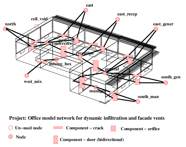
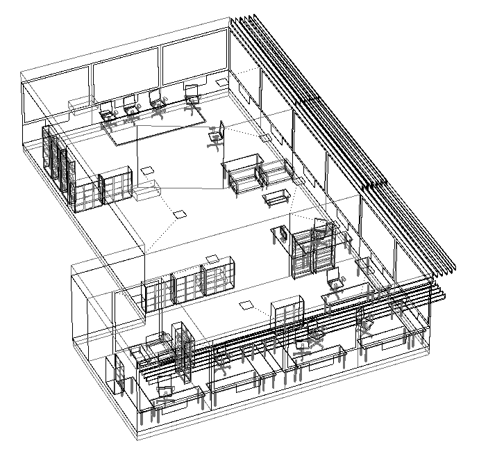


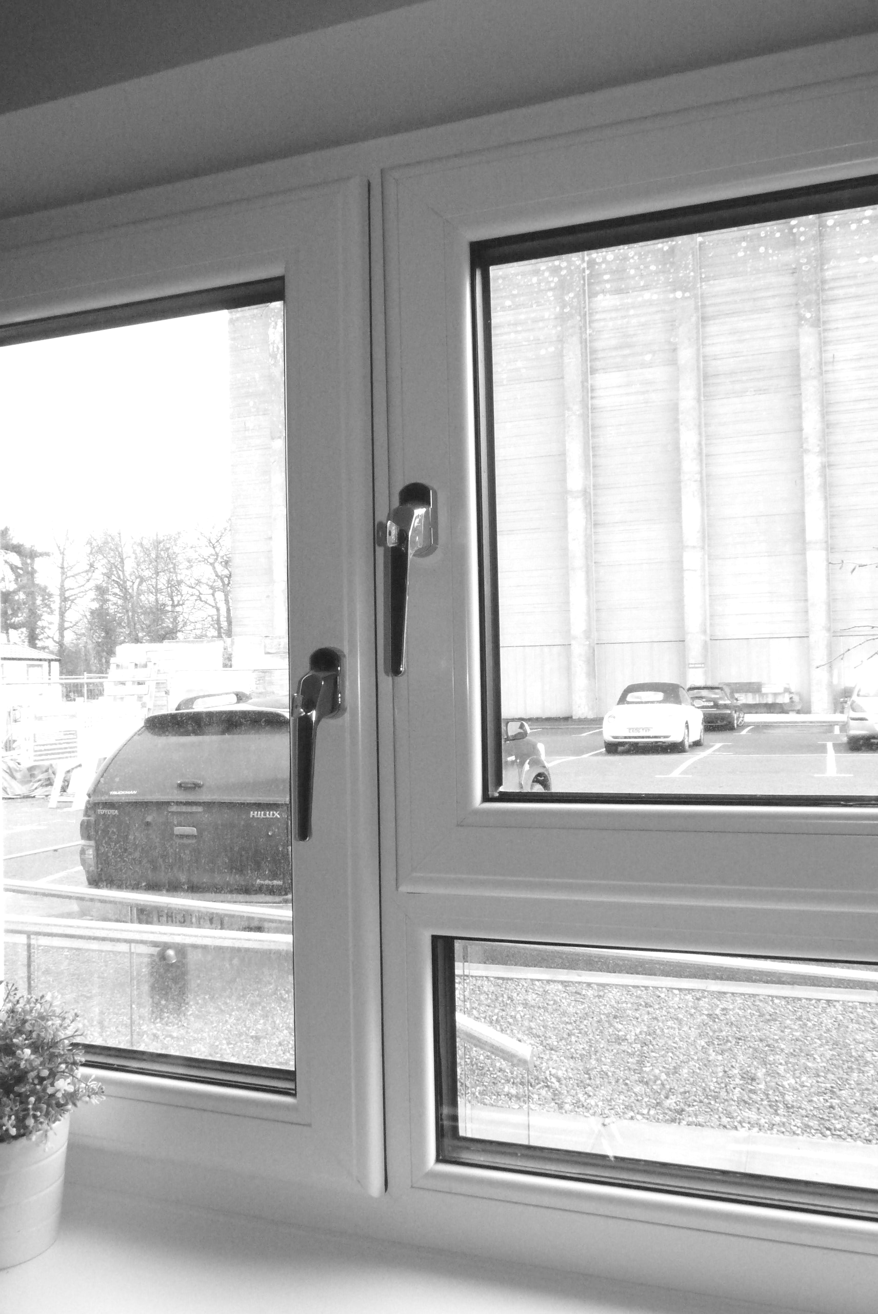

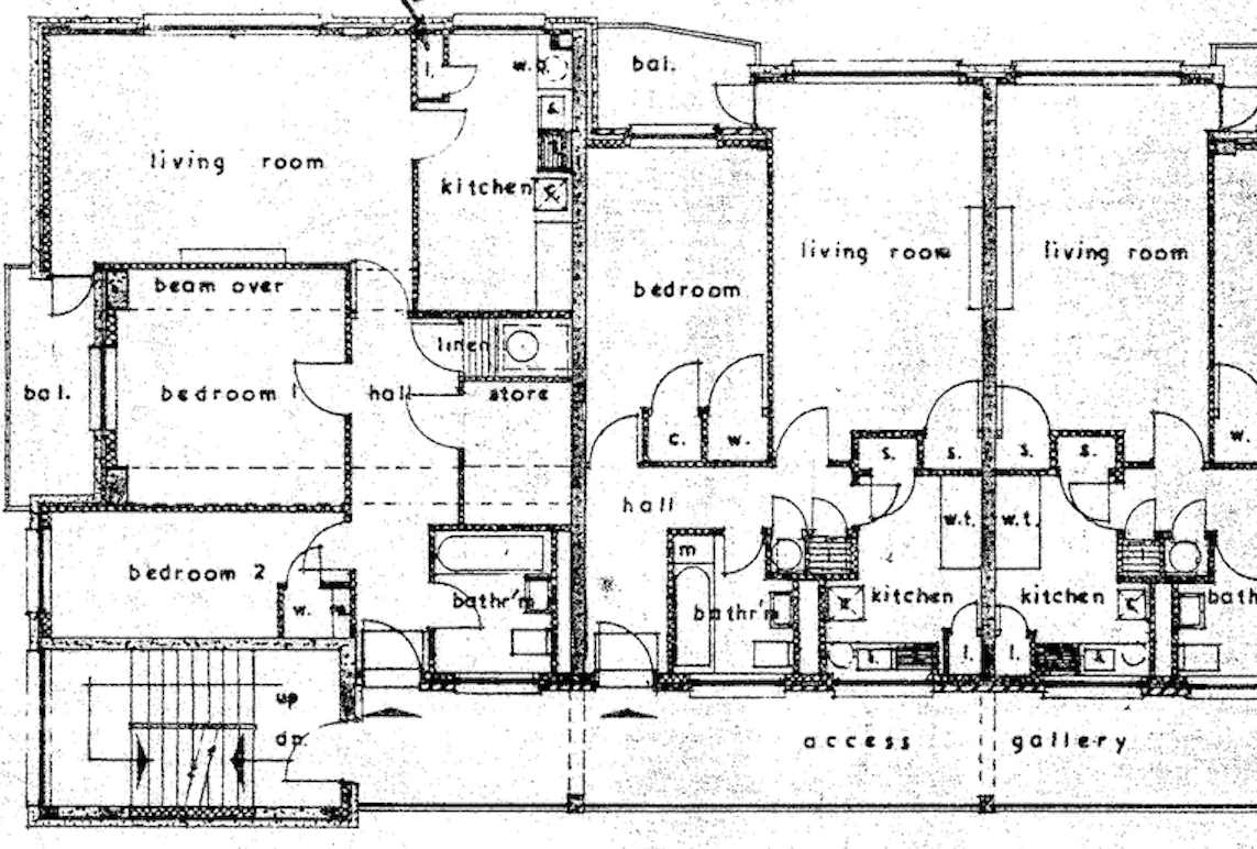
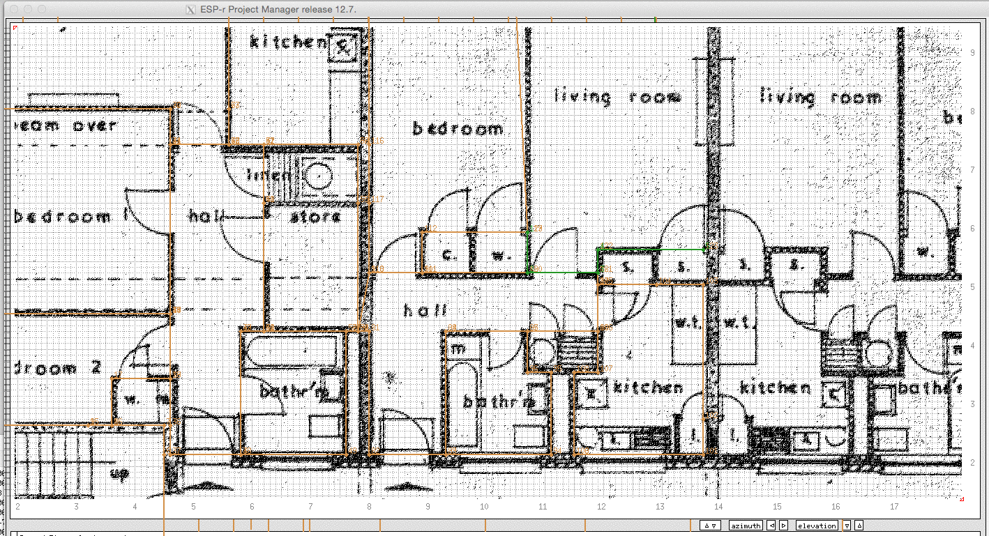
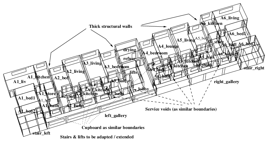
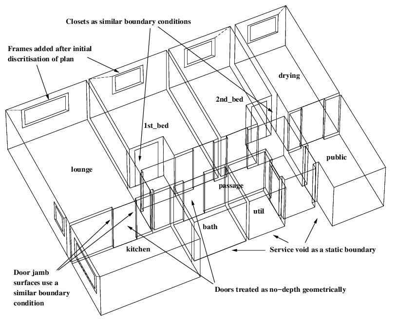
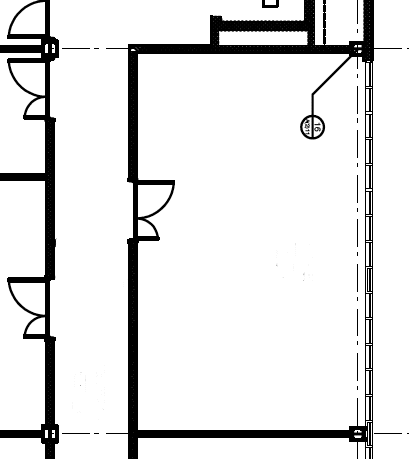
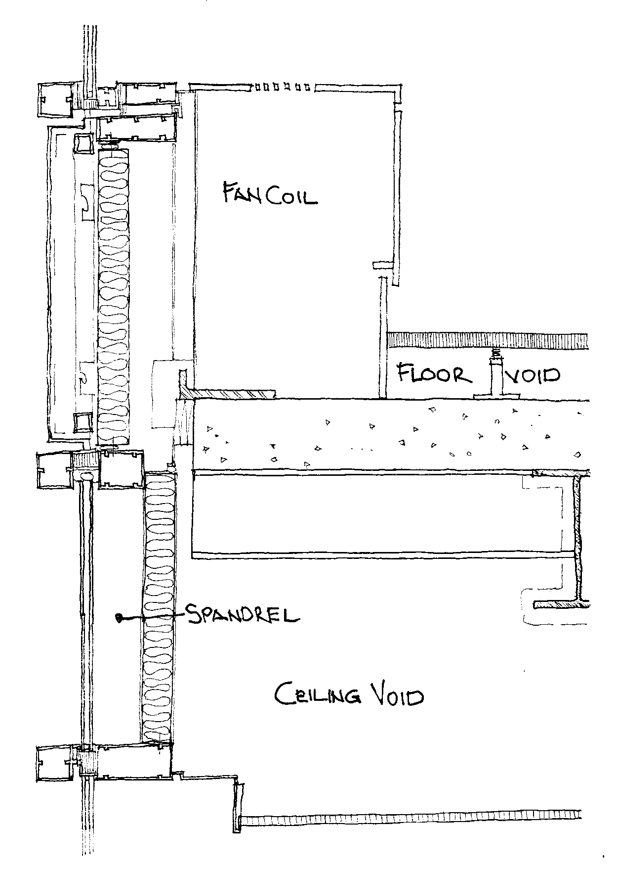
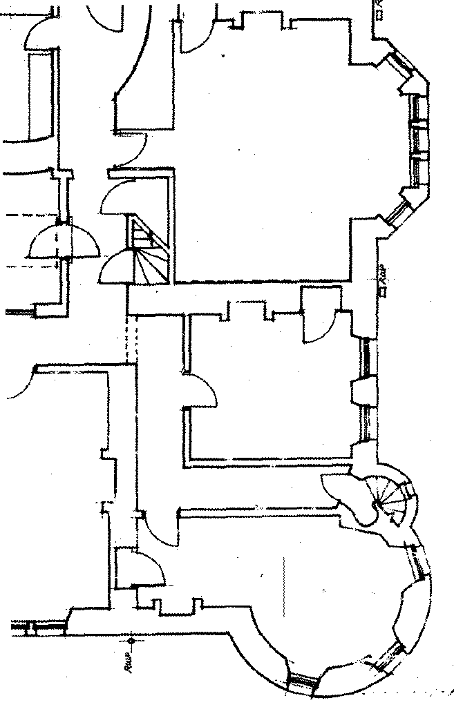

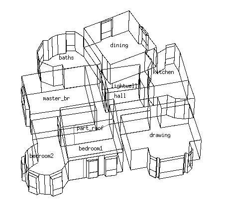
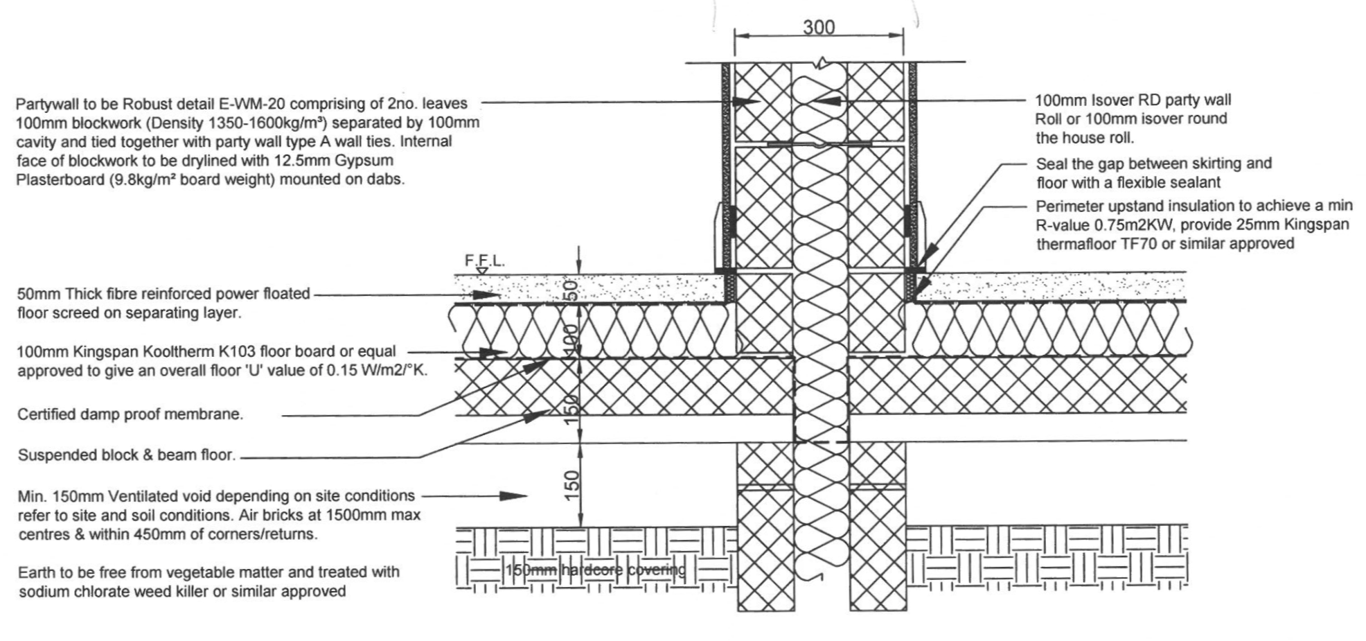
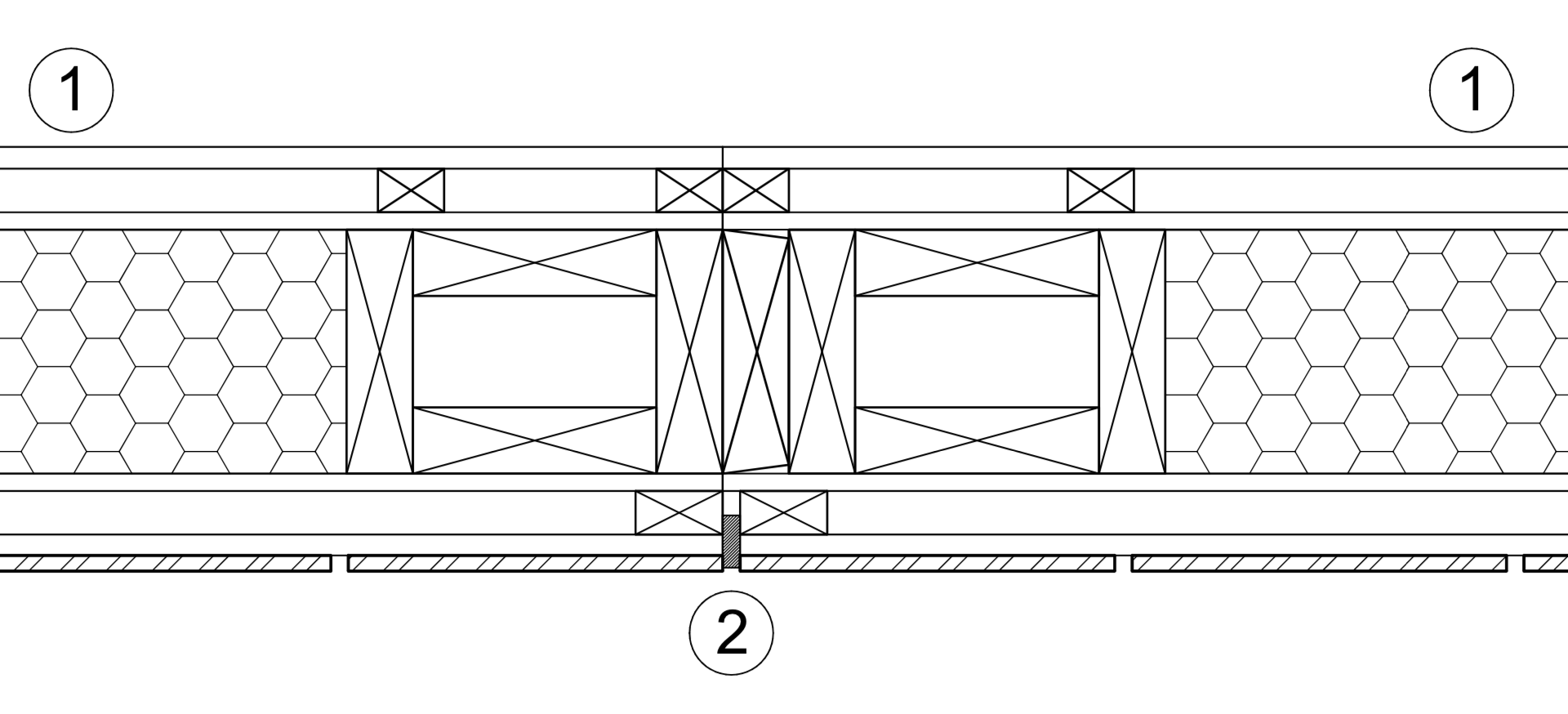
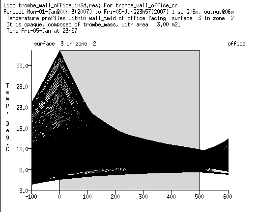
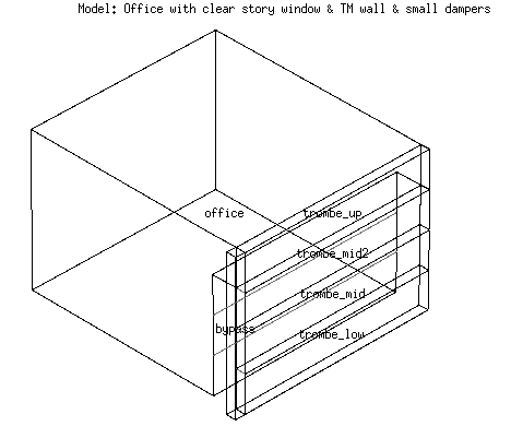
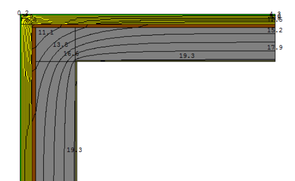
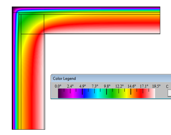
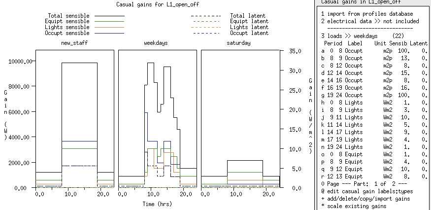
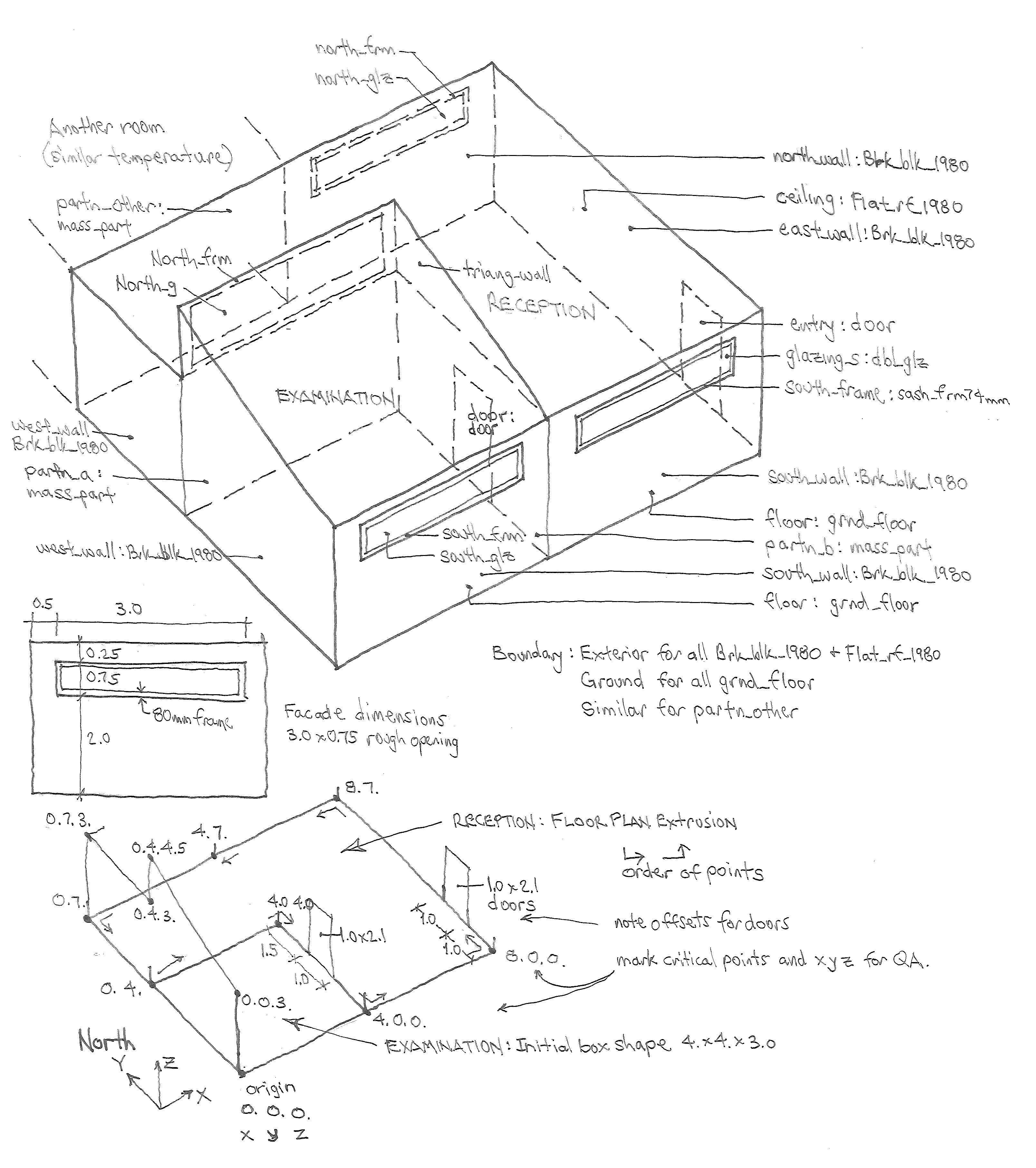


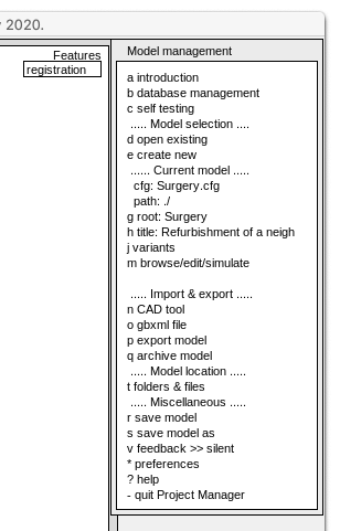
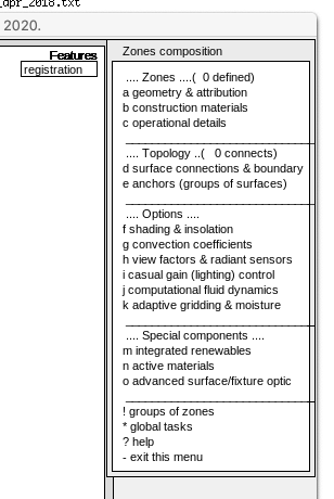
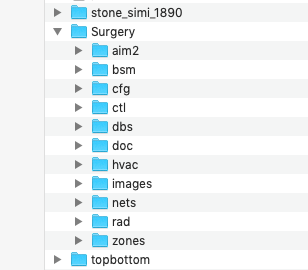
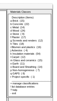
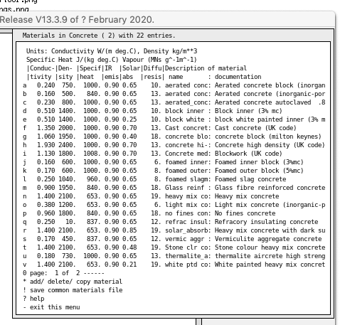

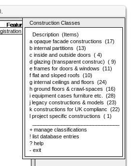
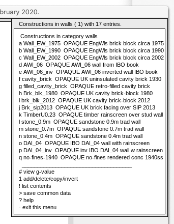
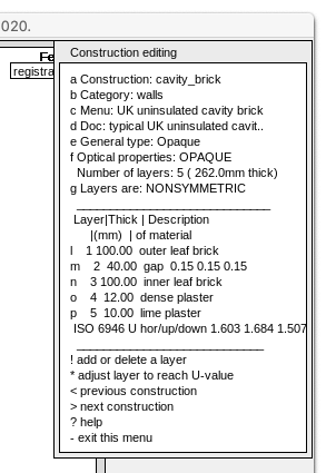
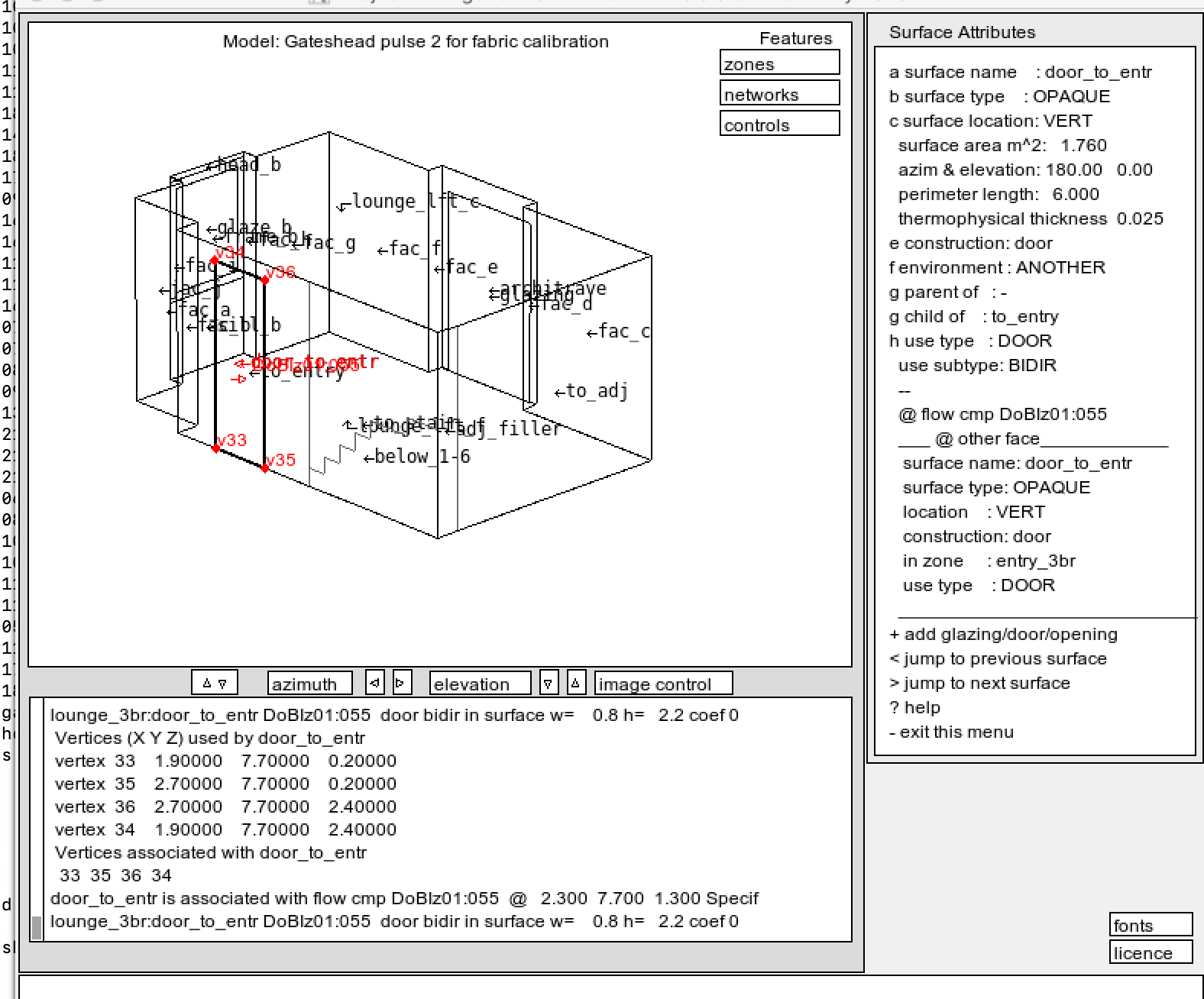

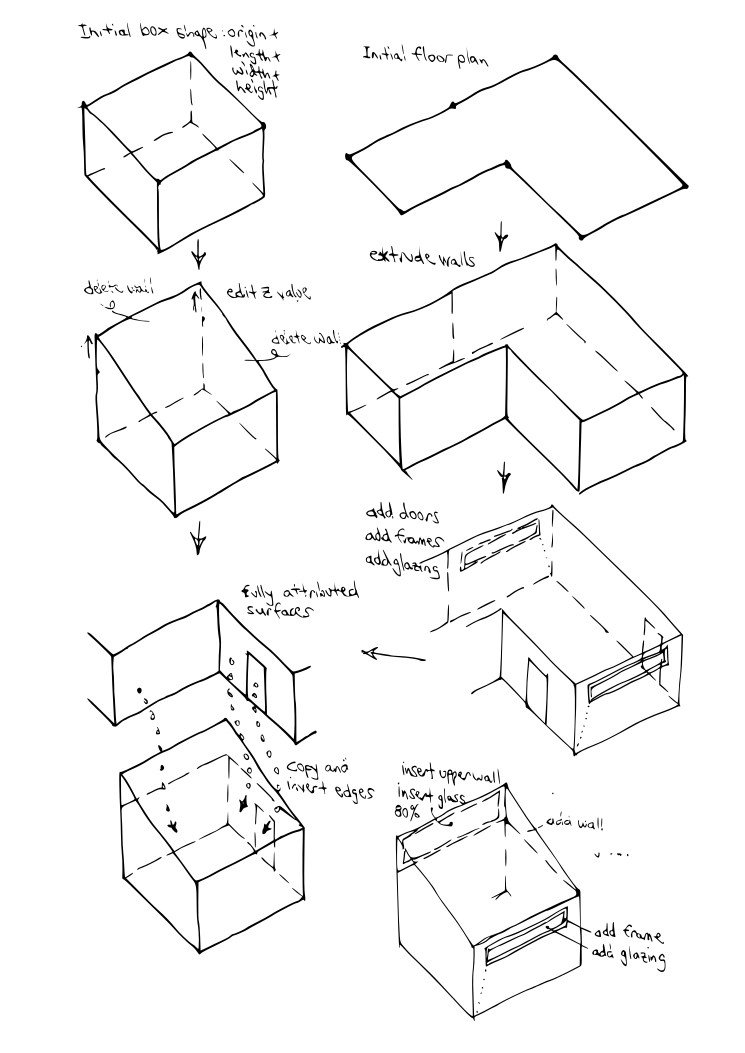
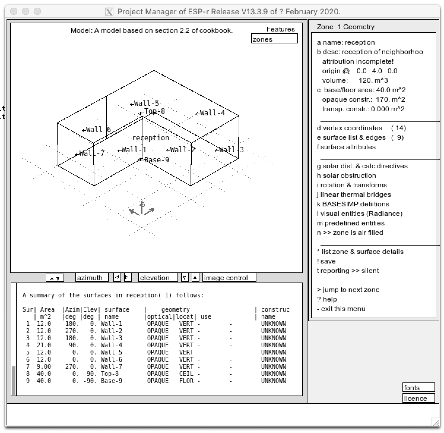

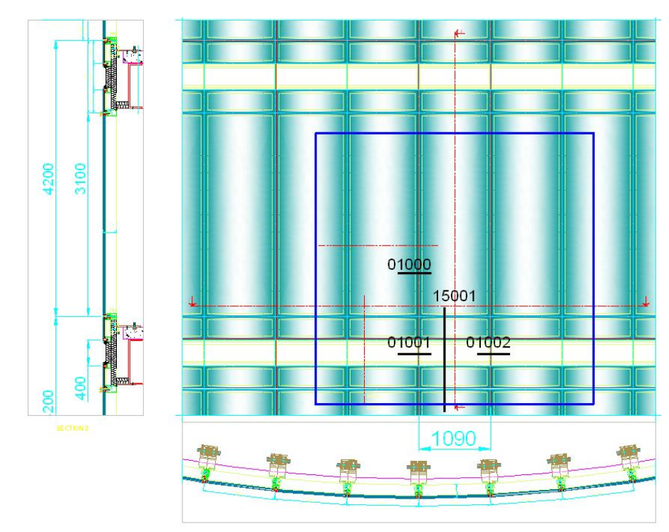
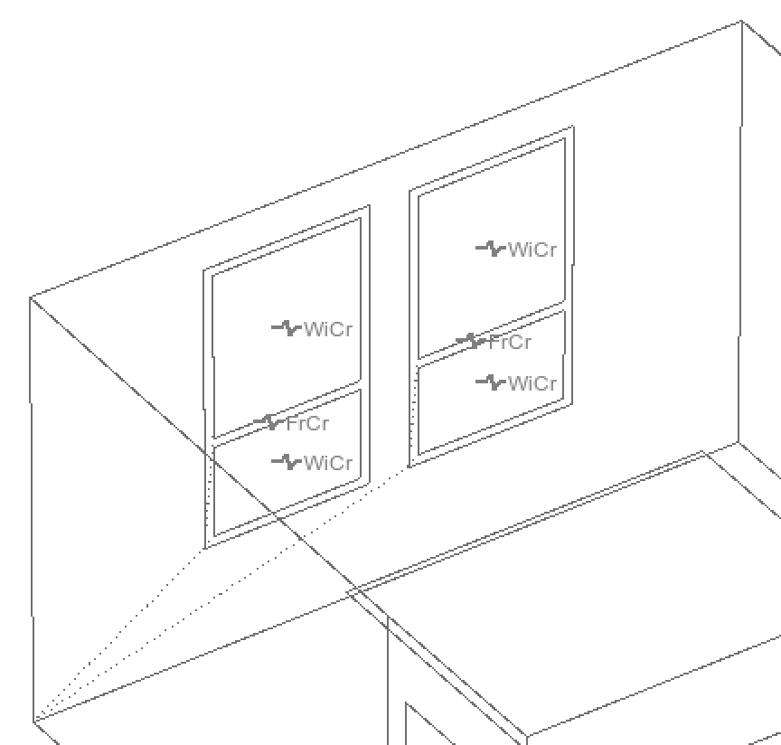

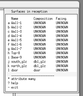
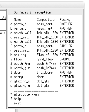

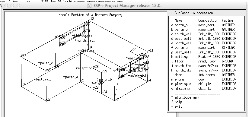
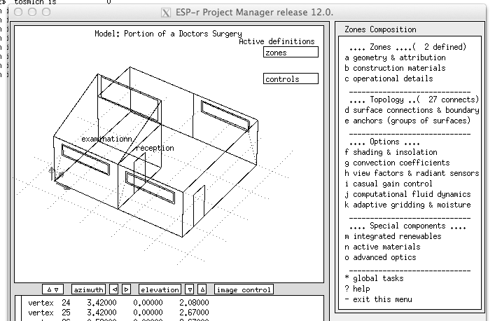
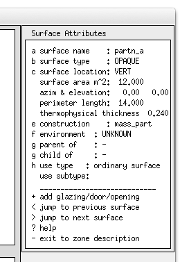
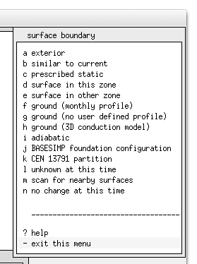


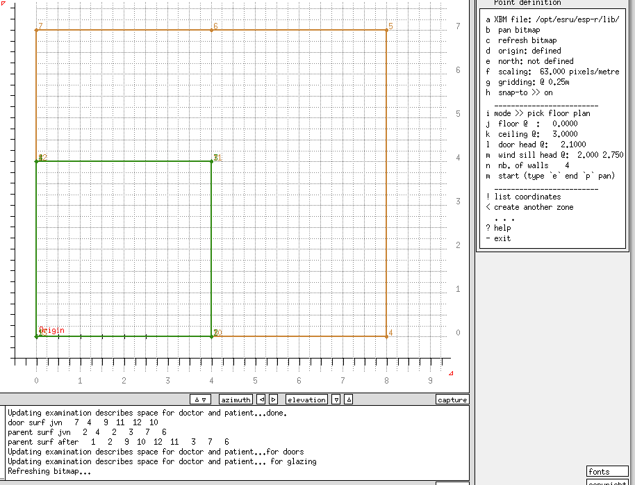
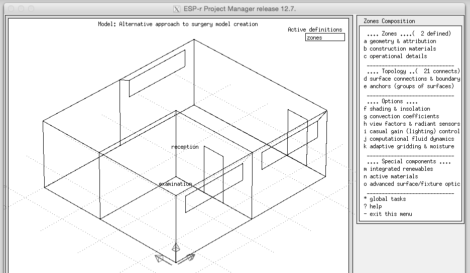

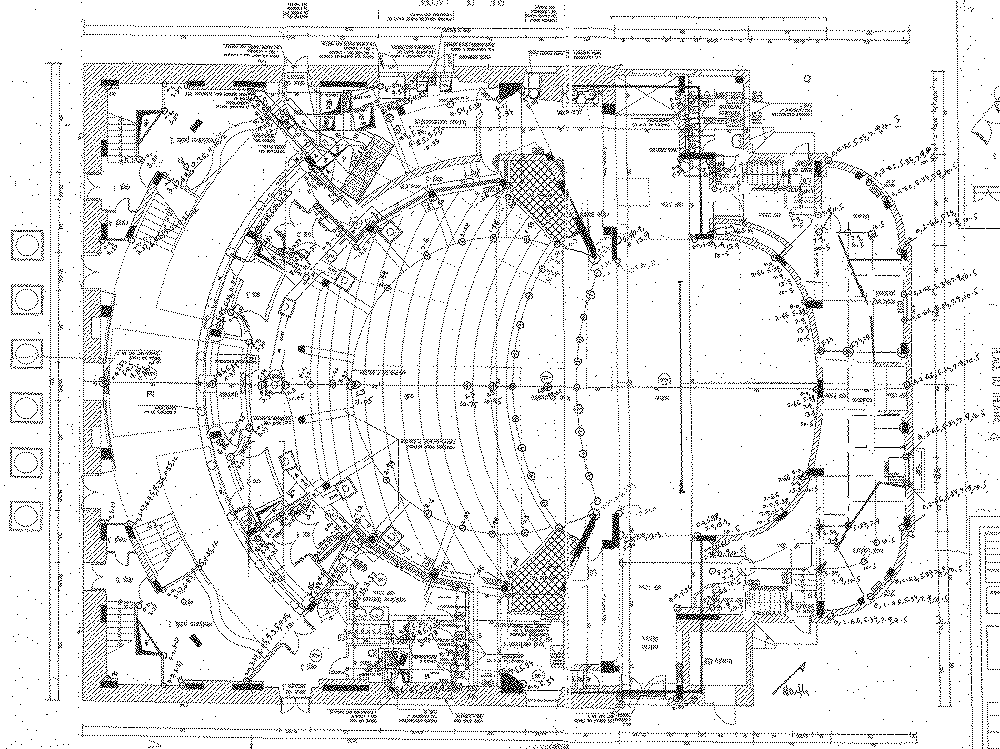

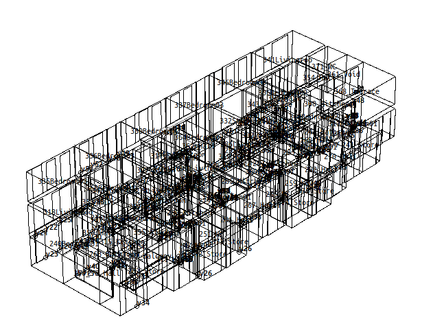
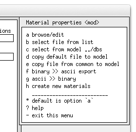
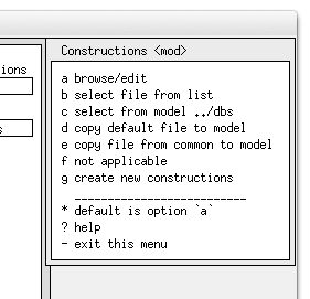
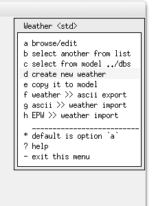
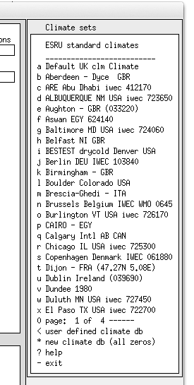
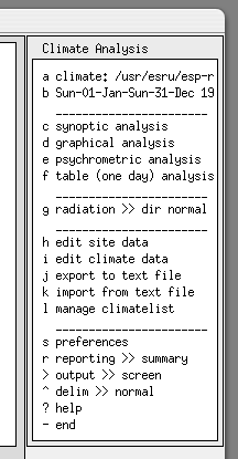
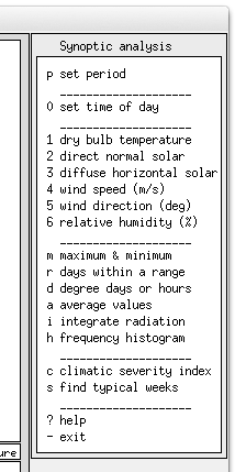
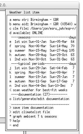
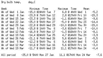
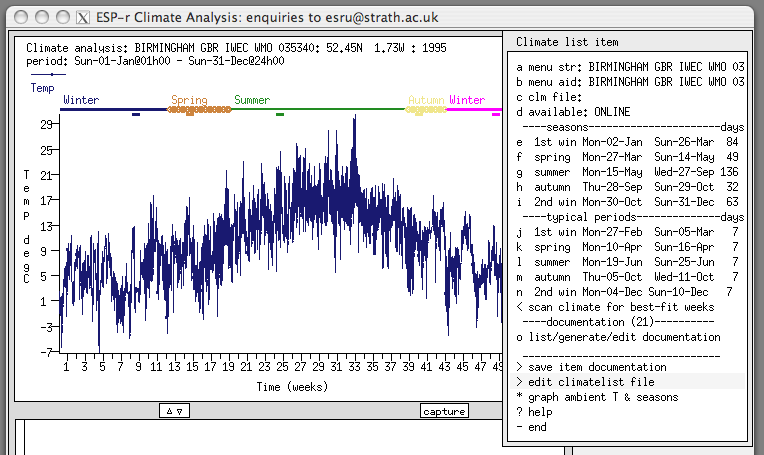
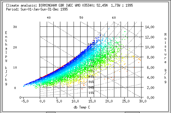


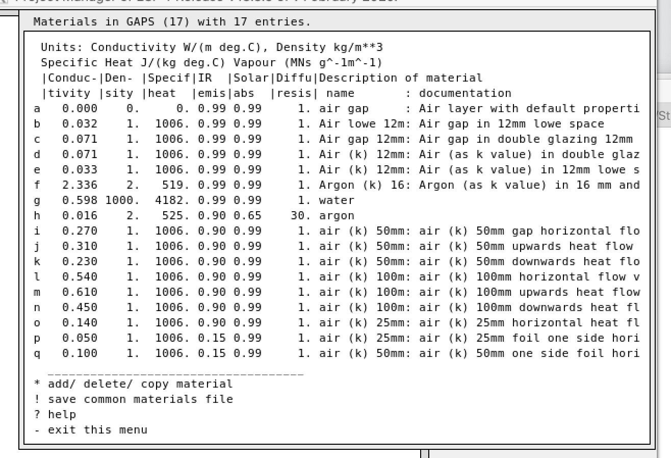


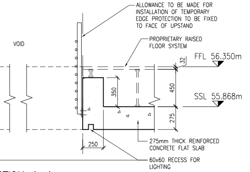
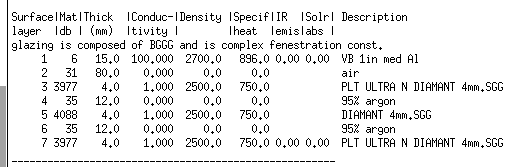
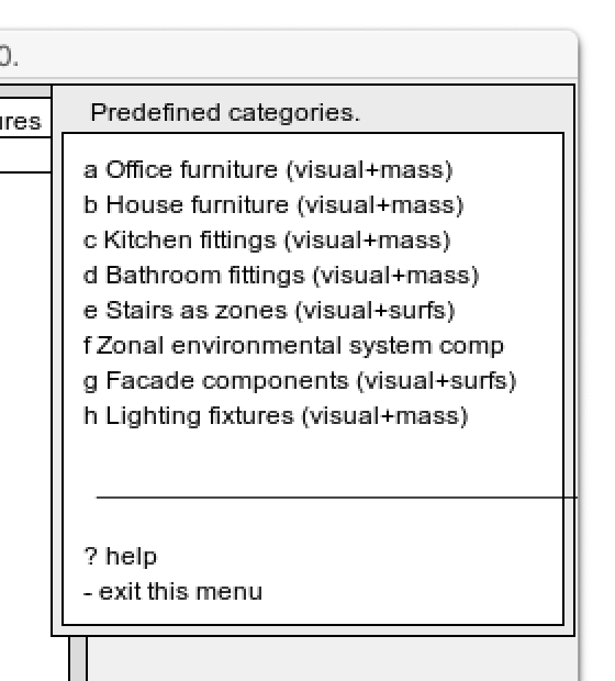
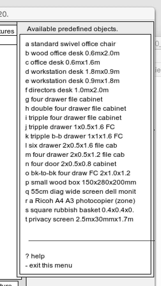
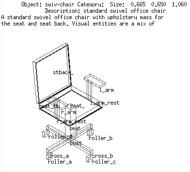
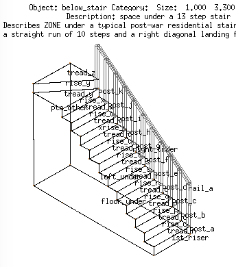
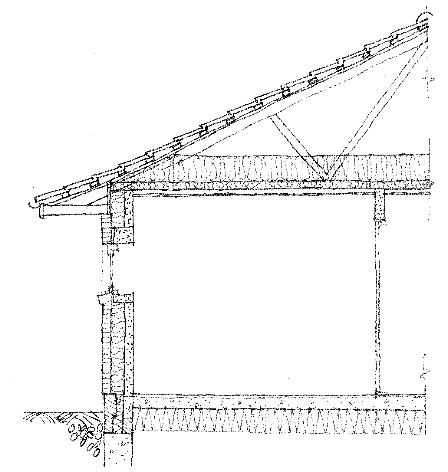
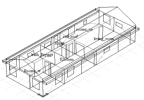
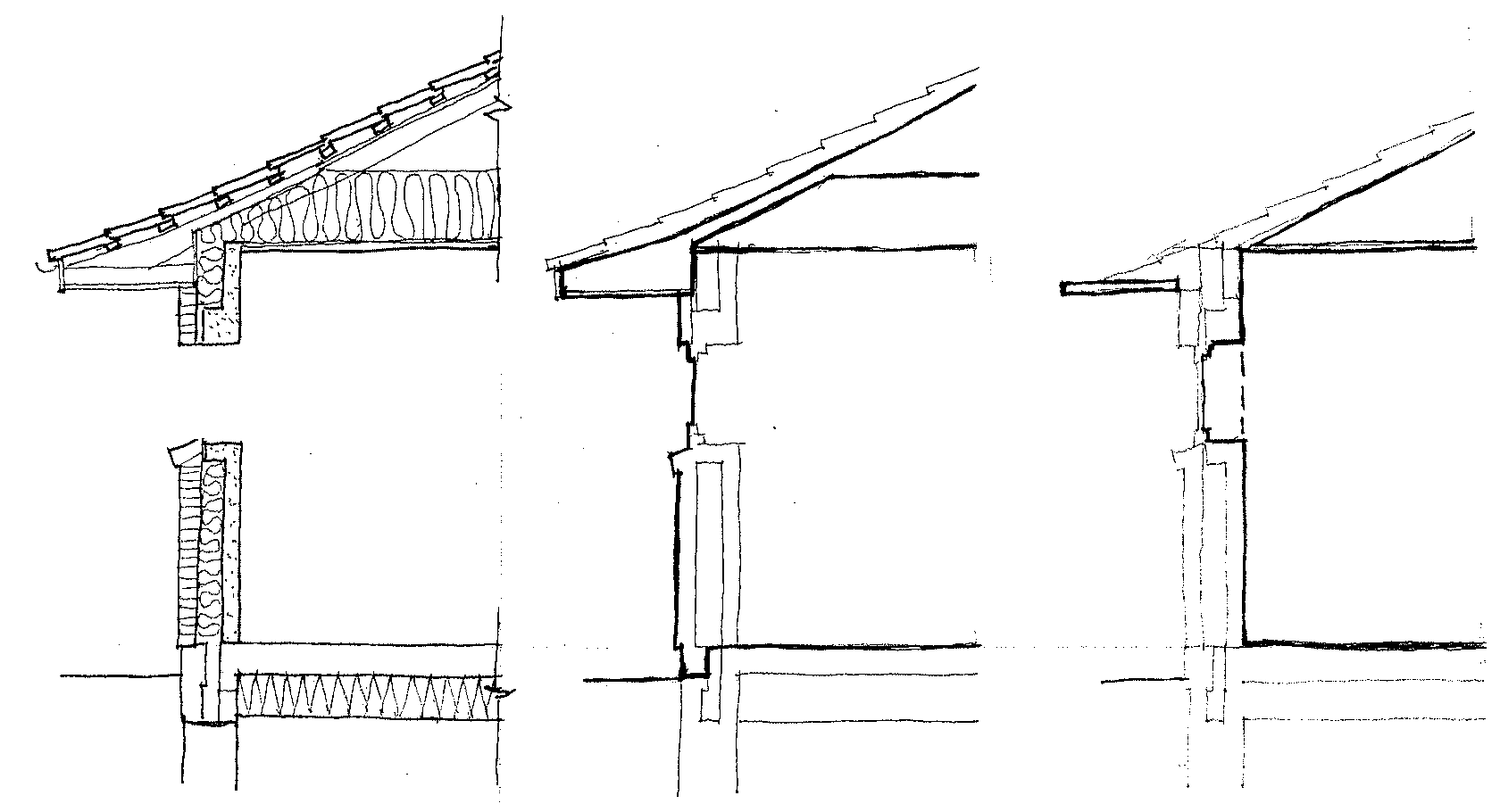
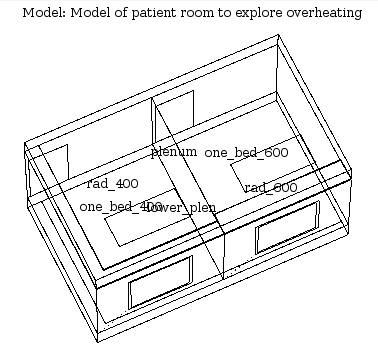
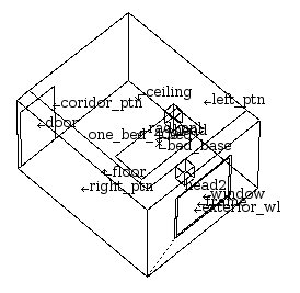
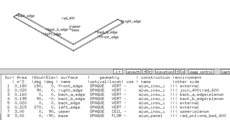
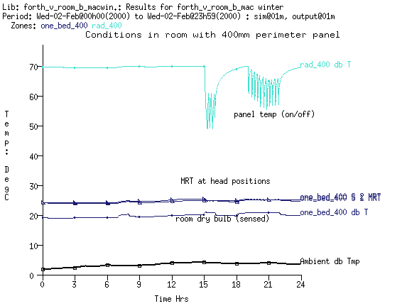
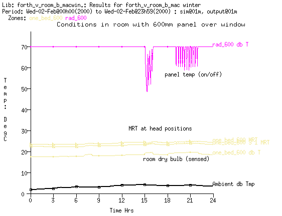
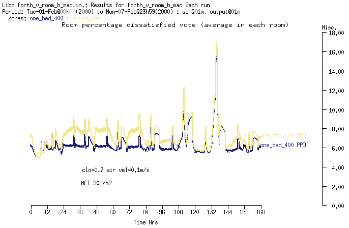

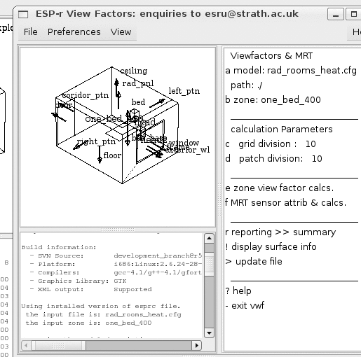
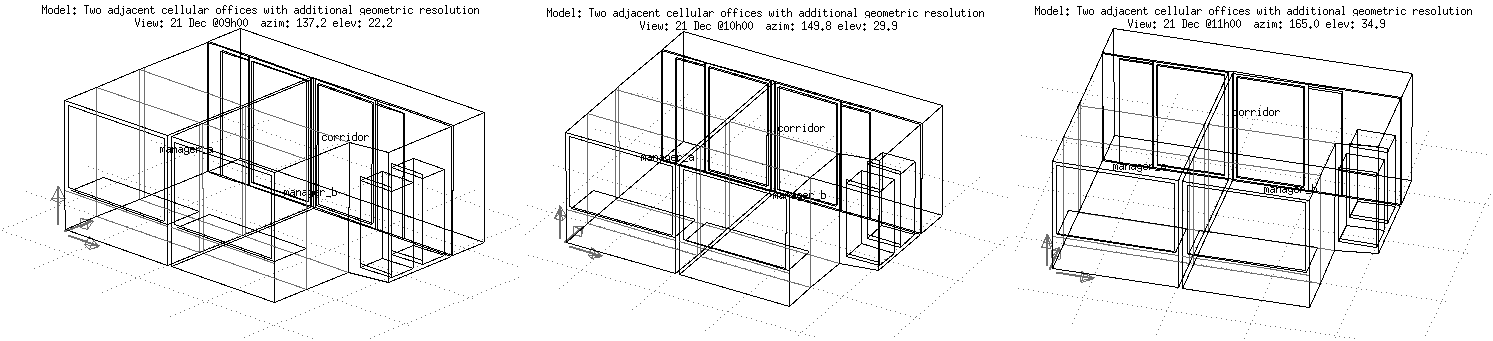
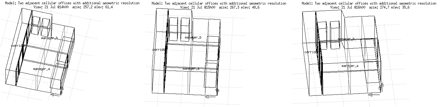
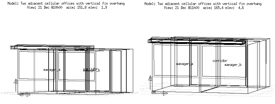
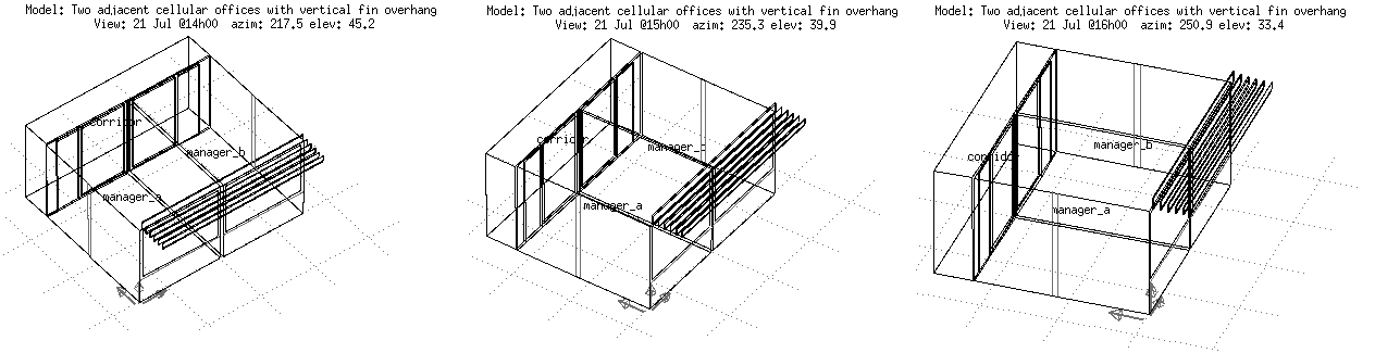

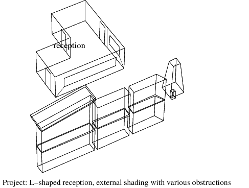

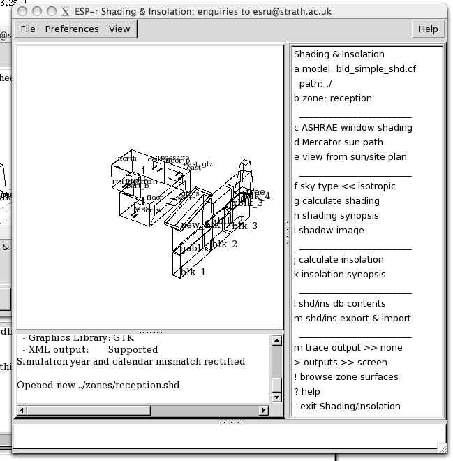

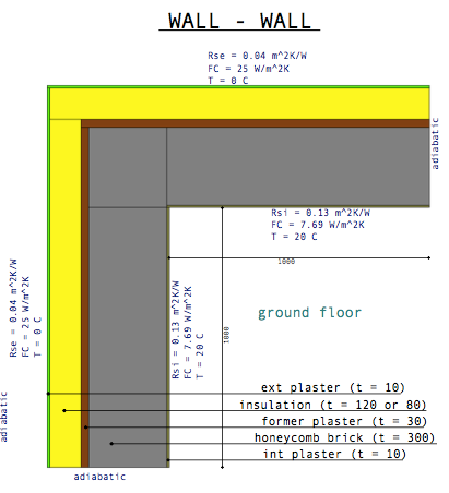
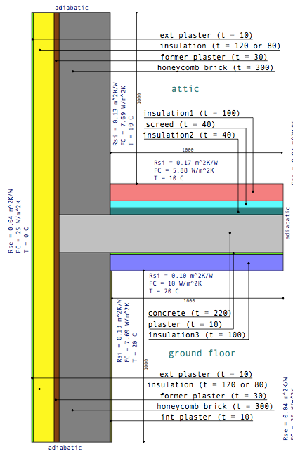
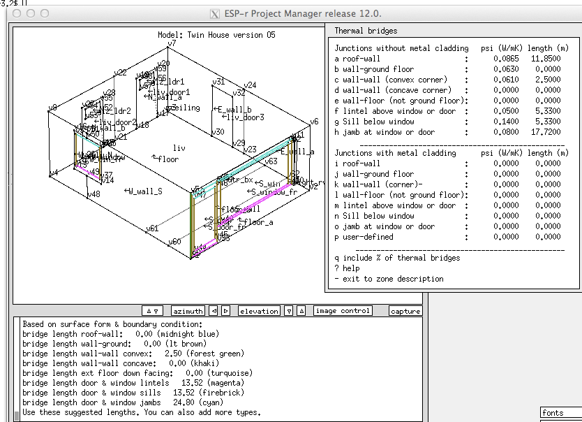
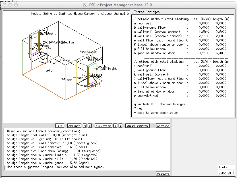
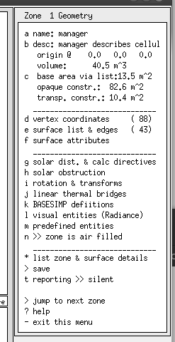
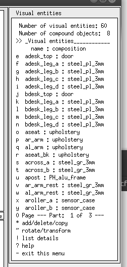
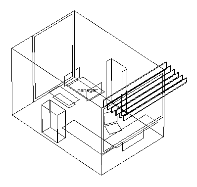
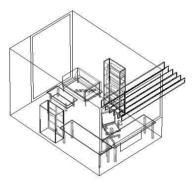
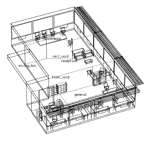
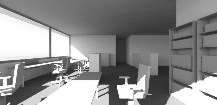
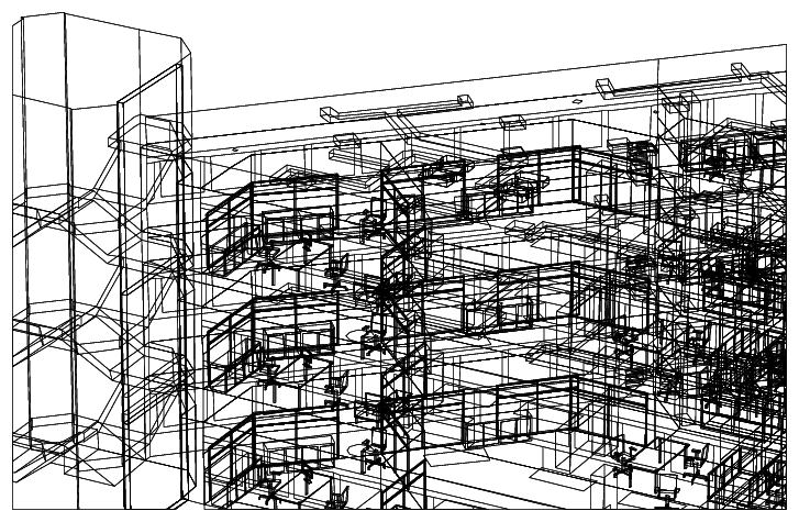
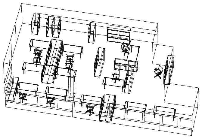

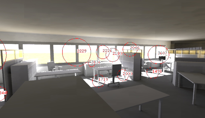
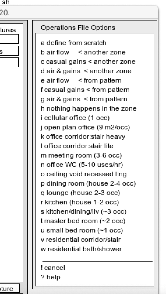


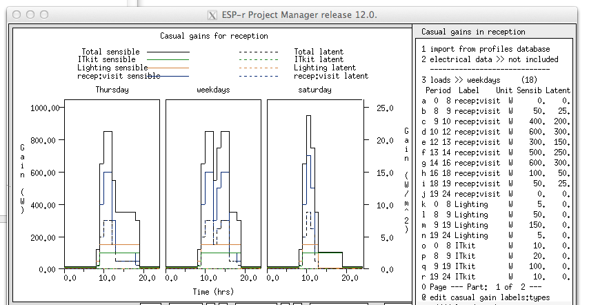
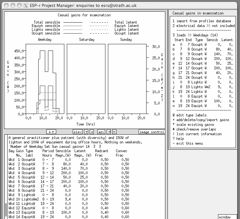
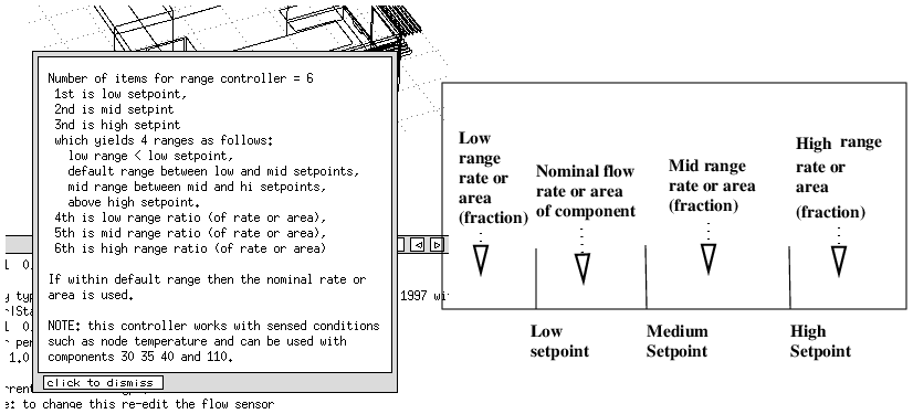
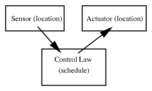

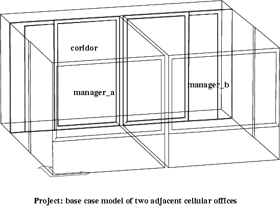
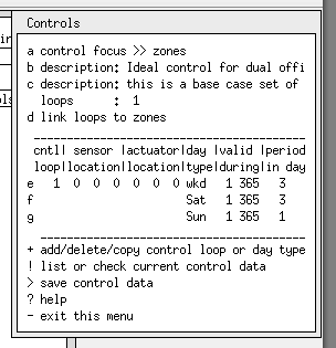 . . .
. . .